Introduction
What is LaTeX
LaTeX (pronounced /ˈlɑːtɛx/ or /ˈleɪtɛx/) is a typesetting system that makes your documents look more professional, rather than a word processor. It is particularly well suited to long, rigorously structured documents and is especially good at typesetting formulas. It is free software and works on most operating systems.
LaTeX is based on TeX, a typesetting system designed by Donald Knuth in 1978 for digital typesetting. TeX is a low-level language that computers can process, but most people find it difficult to use. LaTeX was designed precisely to make it easier to use. The current version of LaTeX is LaTeX 2e.
If you are used to working with documents in Microsoft Office Word, you will find LaTeX's way of working quite unfamiliar. Word is a typical “what you see is what you get” editor: you can see the final layout while arranging the document. With LaTeX, however, you cannot conveniently see the final result as you work, which lets you focus on the content rather than adjusting its appearance.
A LaTeX document is a text file ending in .tex. It can be edited with any text editor, such as Notepad, but for most people, using a suitable LaTeX editor makes the editing process much easier. While editing, you can mark the structure of the document. Once finished, you can compile it—that is, convert it into a document in another format. Several formats are supported, but PDF is the most commonly used.
Before you start
The notation used in this article is listed below:
- Operations that you are expected to perform are marked with an arrow ;
- Characters that you type are enclosed in code blocks;
- Menu commands and button names are marked in bold.
Some concepts
To write LaTeX documents, you need to install a “distribution”. Common distributions include TeX Live, MikTeX, and MacTeX for macOS users (which is actually the macOS version of TeX Live). CTeX is no longer recommended. TeX Live and MacTeX include almost all LaTeX packages, whereas MikTeX includes only a small number of essential packages and installs other packages when they are needed.
TeX Live and MikTeX both include the TeXworks editor. You can also install the more feature-rich TeXstudio editor, or configure an editor such as Visual Studio Code or Notepad++ yourself. The editor used below is TeXworks running on Windows 7.
Most distributions include multiple engines, such as pdfTeX and XeTeX. For Chinese users, XeTeX is recommended for Unicode support.
TeX has several formats, such as Plain TeX and LaTeX. LaTeX format is generally used today, so you need to use the engine packaged with the format you are using. For example, with pdfTeX you need to use pdfLaTeX, and with XeTeX you need to use XeLaTeX.
Further reading: Introduction to TeX engines, formats, and distributions.
Setting up the environment
Windows users need to download TeX Live or MikTeX. Users in mainland China can use the Tsinghua University TUNA mirror. Click the “Get download link” button on the right side of the page, select the “Software” tab, and choose “TeX typesetting system” to download the TeX Live or MikTeX installer. The TeX Live installer is an ISO file; after mounting it, run install-tl-advanced.bat with administrator privileges.
The Tsinghua University TUNA mirror also provides downloads of MacTeX and the macOS version of MikTeX for macOS users.
For Linux users, if you use TeX Live, likewise download the ISO file and run the install-tl script; if you use MikTeX, follow the official documentation to install it.
Document structure
Basic elements
Open TeXworks.
A new document opens automatically.
Open the Format menu and select Line Numbers.
Line numbers are not an essential element, but they can help you compare the code with the information on the screen and find errors.
Open the Format menu, select Syntax Coloring, and then select LaTeX.
Syntax coloring highlights the code, making it easier to read.
Enter the following text:
\documentclass[a4paper, 12pt]{article}

\begin{document}
  A sentence of text.
\end{document}
The \documentclass command must appear at the beginning of every LaTeX document. The text inside the braces specifies the document type. The article document type is suitable for shorter articles, such as journal articles and short reports. Other document types include report (for longer, multi-chapter documents such as doctoral theses), proc (conference proceedings), book, and beamer. The text inside the square brackets specifies some options—in this example, the paper size is set to A4 and the main text size to 12pt.
The \begin{document} and \end{document} commands wrap the content of your document. Any text before \begin{document} is treated as preamble commands and affects the entire document. Any text after \end{document} is ignored.
Blank lines are not necessary, but they make long documents easier to read.
Press the Save button; create a folder named LaTeX course in Libraries>Documents; name your document Doc1 and save it as a TeX document in this folder.
It is a good idea to put different LaTeX documents in different directories and combine multiple files when compiling.
Make sure the typeset menu is set to xeLaTeX. Click the Typeset button.
Your source file is now converted into a PDF document, which takes some time. When compilation is complete, the TeXworks PDF viewer opens and previews the generated file. The PDF file is automatically saved in the same directory as the TeX document.
Dealing with problems
If your document contains an error and TeXworks cannot create a PDF document, the Typeset button turns into a red cross and the terminal output at the bottom remains expanded. Then:
Click the Abort typesetting button. Read the terminal output; the last line may give the line number where the error occurred. Find the corresponding line in the document and fix the error. Click the Typeset button again to try compiling the source file.
Adding a document title
The \maketitle command creates a title for the document. You need to specify the document title. If no date is specified, the current date is used; the author is optional.
Immediately after \begin{document} and the command, enter the following text:
\title{My First Document}
\author{My Name}
\date{\today}
\maketitle
Your document now looks like this:
\documentclass[a4paper, 12pt]{article}

\begin{document}
  \title{My First Document}
  \author{My Name}
  \date{\today}
  \maketitle

  A sentence of text.
\end{document}
Click the Typeset button and check the generated PDF document.
Key points:
\todayinserts the current date. You can also enter a different date, such as\date{November 2013}.- The body of an article document is typeset on the same page immediately after the title. report places the title on a separate page.
Sections
If needed, you may want to divide your document into chapters (Chapters), sections (Sections), and subsections (Subsections). The following sectioning commands apply to article documents:
\section{...}\subsection{...}\subsubsection{...}\paragraph{...}\subparagraph{...}
The text inside the braces is the section title. For report and book documents, the \chapter{...} command is also supported.
Replace “A sentence of text.” with the following text:
\section{Introduction}
This is the introduction.

\section{Methods}

\subsection{Stage 1}
The first part of the methods.

\subsection{Stage 2}
The second part of the methods.

\section{Results}
Here are my results.
Your document becomes:
\documentclass[a4paper, 12pt]{article}

\begin{document}
  \title{My First Document}
  \author{My Name}
  \date{\today}
  \maketitle

  \section{Introduction}
  This is the introduction.

  \section{Methods}

  \subsection{Stage 1}
  The first part of the methods.

  \subsection{Stage 2}
  The second part of the methods.

  \section{Results}
  Here are my results.
\end{document}
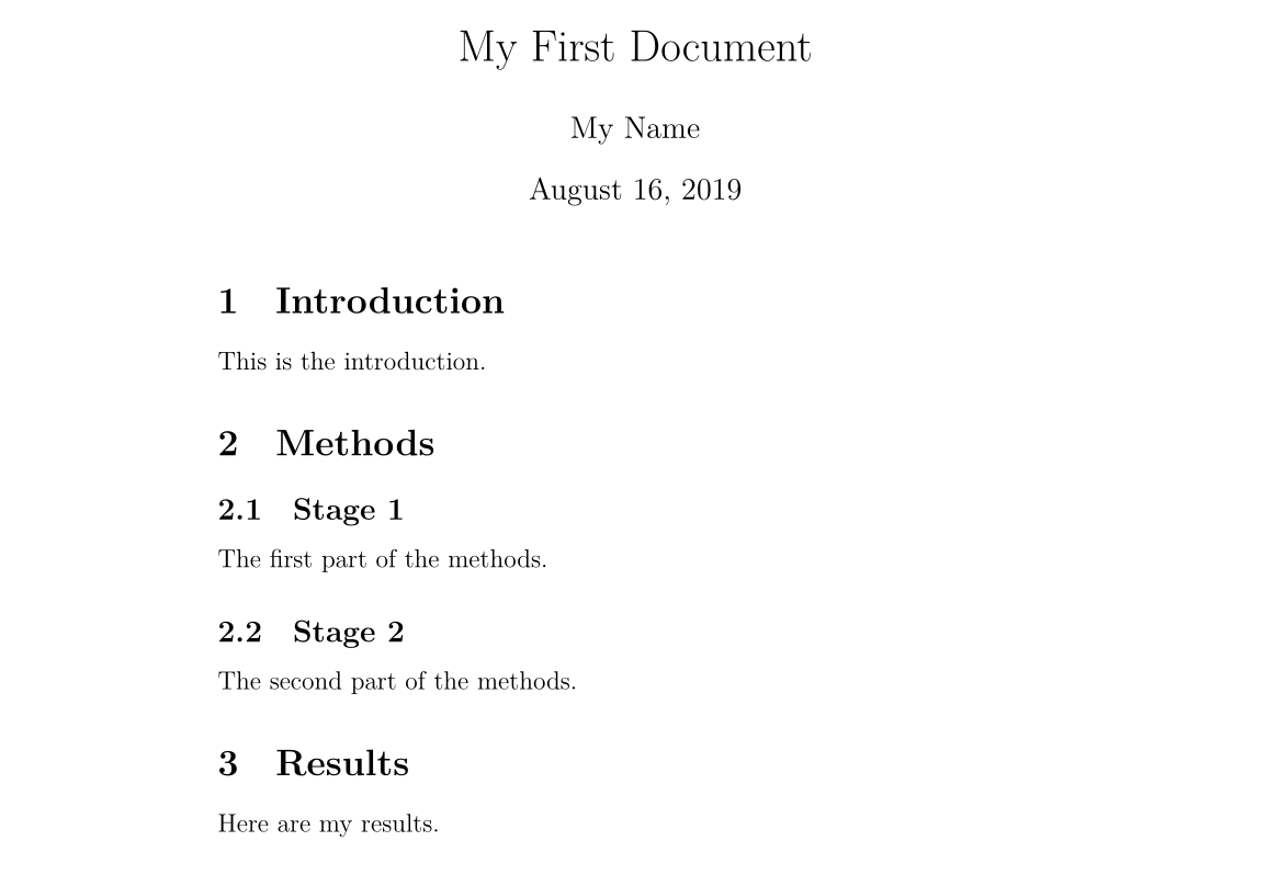
Click the Typeset button and check the PDF document. It should look like this:
Creating labels
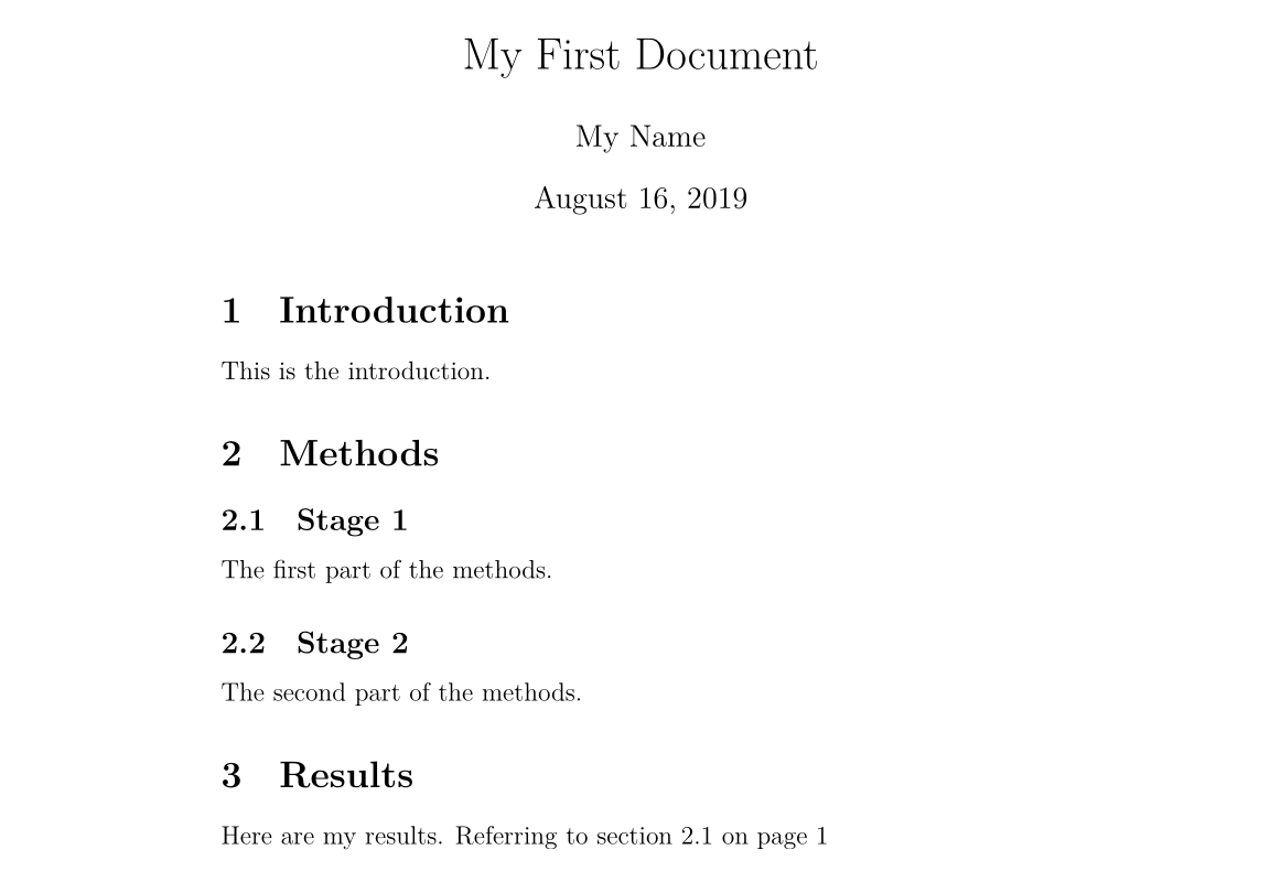
You can create labels for any sectioning command and refer to them elsewhere in the document. Use \label{labelname} to label a section, then enter \ref{labelname} or \pageref{labelname} to refer to the corresponding section.
On a new line below \subsection{Stage 1}, enter \label{sec1}. In the Results section, enter Referring to section \ref{sec1} on page \pageref{sec1}.
Your document becomes:
\documentclass[a4paper, 12pt]{article}

\begin{document}
  \title{My First Document}
  \author{My Name}
  \date{\today}
  \maketitle

  \section{Introduction}
  This is the introduction.

  \section{Methods}

  \subsection{Stage 1}
  \label{sec1} The first part of the methods.

  \subsection{Stage 2}
  The second part of the methods.

  \section{Results}
  Here are my results. Referring to section \ref{sec1} on page \pageref{sec1}
\end{document}
Compile and check the PDF document (you may need to compile it twice):
Generating a table of contents (TOC)
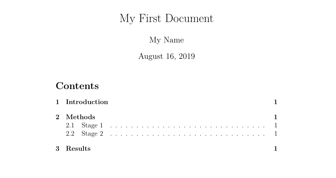
If you use sectioning commands, you can easily generate a table of contents. Use \tableofcontents to create a table of contents in the document. It is usually placed after the title.
You may also want to change the page numbers to Roman numerals (i,ii,iii). This ensures that the body of the document starts on page 1. Page numbering can be switched between Arabic and Roman numerals with \pagenumbering{...}.
Enter the following after \maketitle:
\pagenumbering{roman}
\tableofcontents
\newpage
\pagenumbering{arabic}
The \newpage command starts a new page, allowing us to see the effect of the \pagenumbering command. The first 14 lines of your document look like this:
\documentclass[a4paper, 12pt]{article}

\begin{document}

\title{My First Document}
\author{My Name}
\date{\today}
\maketitle

\pagenumbering{roman}
\tableofcontents
\newpage
\pagenumbering{arabic}
Compile and check the document (you may need to compile it several times; this will not be repeated below).
The first page of the document looks like this:
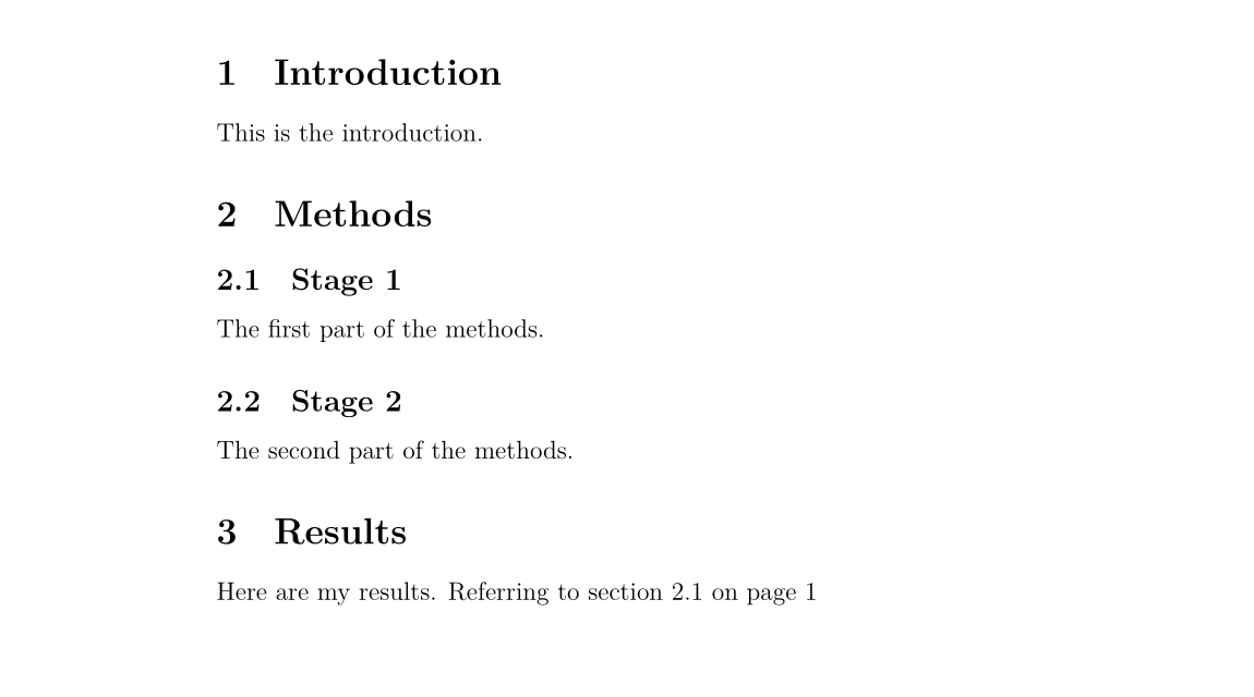
The second page:
Text processing
Support for Chinese fonts
For readers studying LaTeX, the first thing to learn is naturally LaTeX's support for Chinese fonts. In fact, there are many ways to make LaTeX support Chinese fonts. Here we give only the most concise solution: use the CTeX package. Simply add the following to the preamble of the document:
\usepackage[UTF8]{ctex}
That is all. Compile the document with the xelatex command, because it supports Chinese fonts.
Font effects
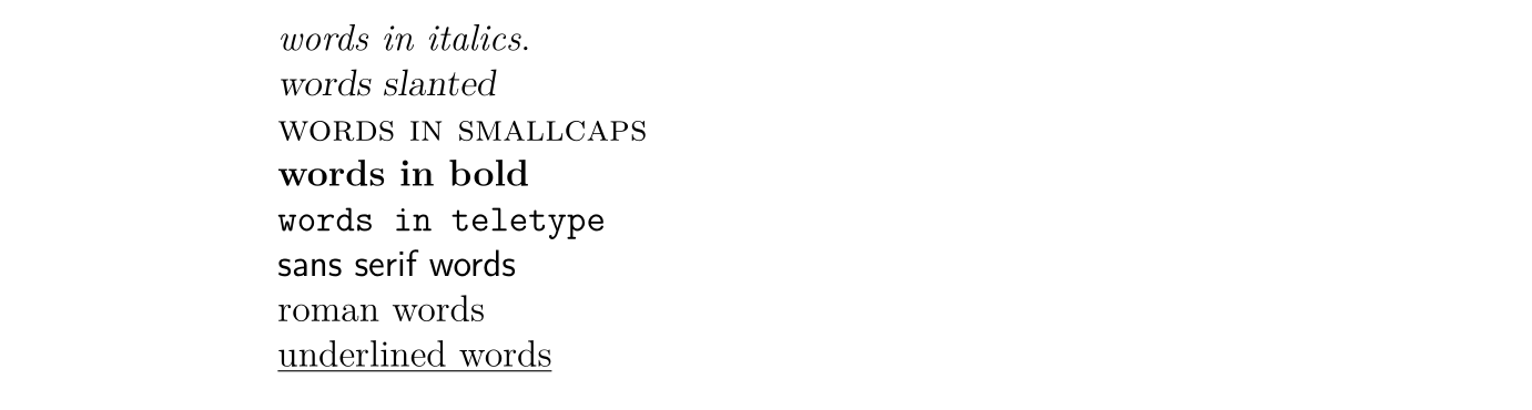
LaTeX has many different font effects; some are listed here:
\textit{words in italics} \textsl{words slanted} \textsc{words in smallcaps} \textbf{words
in bold} \texttt{words in teletype} \textsf{sans serif words} \textrm{roman
words} \underline{underlined words}
The result is as follows:
Add more text to your document and try the various font effects.
Colored text
To make your document support colored text, you need to use a package. You can load many packages to enhance LaTeX's typesetting. Package-loading commands are placed in the document preamble (that is, before the \begin{document} command). Use \usepackage[options]{package} to load a package. Here package is the name of the package, and options are parameters specifying its features.
After using \usepackage{color}, we can use common colors:

The code for colored text is:
{\color{colorname}text}
Here colorname is the name of the color you want, and text is the content of your colored text. Notice that the yellow and white in the example have a text background color; this can likewise be achieved with the \colorbox command from the Color package. Its usage is as follows:
\colorbox{colorname}{text}
Before \begin{document}, enter \usepackage{color}. Enter {\color{red}fire} in the document content. Compile and check the PDF document.
The word fire should be red.
You can add parameters to use more colors, and even define the colors you need. This is beyond the scope of this book. For more information about colored text, read the Colors chapter of the LaTeX Wikibook.
Font sizes
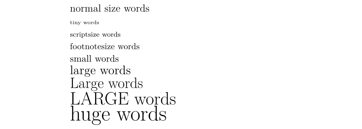
Next, we list some LaTeX commands for setting font sizes:
normal size words {\tiny tiny words} {\scriptsize scriptsize words}
{\footnotesize footnotesize words} {\small small words} {\large large words}
{\Large Large words} {\LARGE LARGE words} {\huge huge words}
The result is as follows:
Try adjusting the font size of your text.
Paragraph indentation
By default, LaTeX leaves the first line of the first paragraph of each section flush left and indents the first line of subsequent paragraphs. To make a paragraph flush left, add the \noindent command before that paragraph. To make all paragraphs flush left globally, use the \setlength{\parindent}{0pt} command at some point in the document; all subsequent paragraphs will be flush left.
Lists
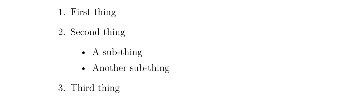
LaTeX supports two types of lists: ordered lists (enumerate) and unordered lists (itemize). Elements in a list are defined with \item. Lists can have sublists.
Enter the following to create an ordered list containing an unordered sublist:
\begin{enumerate}
  \item First thing

  \item Second thing
    \begin{itemize}
      \item A sub-thing

      \item Another sub-thing
    \end{itemize}

  \item Third thing
\end{enumerate}
Compile and check the PDF document.
The list looks like this:
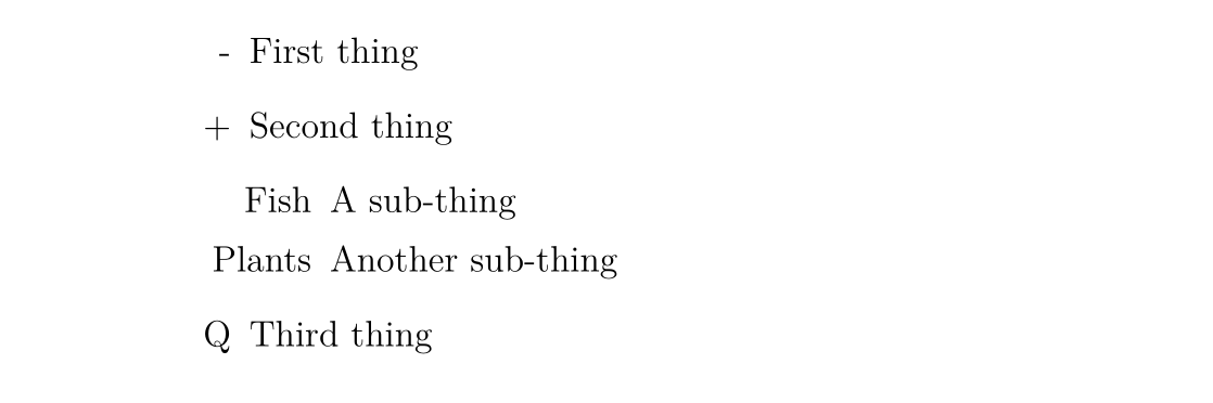
Square-bracket options can be used to change the marker at the head of an unordered list. For example, \item[-] uses a dash as the marker; you can even use a word, such as \item[One].
The following code:
\begin{itemize}
  \item[-] First thing

  \item[+] Second thing
    \begin{itemize}
      \item[Fish] A sub-thing

      \item[Plants] Another sub-thing
    \end{itemize}

  \item[Q] Third thing
\end{itemize}
produces the following result:
Comments and spaces
We use % to create a single-line comment. Everything on that line after this character is ignored until the next line begins.
The following code:
It is a truth universally acknowledged% Note comic irony
in the very first sentence , that a single man in possession of a good fortune,
must be in want of a wife.
produces the following result:

Multiple consecutive spaces are treated as one space in LaTeX. Multiple consecutive blank lines are treated as one blank line. The main purpose of a blank line is to start a new paragraph. In general, LaTeX ignores blank lines and other whitespace; two backslashes (\\) can be used to insert a line break.
Try adding comments and blank lines to your document.
If you want to add space to your document, you can use the \vspace{...} command. This adds vertical space whose height can be specified. For example, \vspace{12pt} produces a space with a height equal to the height of 12pt text.
Special characters
The following characters are special characters in LaTeX:
# $ % ^ & _ { } ~ \
To use these characters, we need to escape them by adding a backslash before each one:
\# \$ \% \^{} \& \_ \{ \} \~{}
When using the ^ and ~ characters, note that a pair of closing braces must immediately follow them; otherwise they are interpreted as superscripts of letters. For example, \^ e becomes . The code above produces the following result:

Note that a backslash cannot be escaped with another backslash (otherwise it becomes a line break); use the \textbackslash command instead.
Enter code to generate the following content in your document:

Ask an expert or consult the source code of this page for help.
Tables
The (tabular) command is used to typeset tables. By default, LaTeX tables have no horizontal or vertical rules—you must set them manually if you need them. LaTeX automatically sets the table width based on its contents. The following code creates a table:
\begin{tabular}{...}
The ellipsis is replaced by the code defining the table's columns:
ldenotes a left-aligned column;rdenotes a right-aligned column;cdenotes a center-aligned column;|denotes a vertical line in a column;
For example, {lll} produces a three-column table with left alignment and no explicit vertical lines; {|l|l|r|} produces a three-column table whose first two columns are left-aligned and whose last column is right-aligned, with explicit vertical lines between adjacent columns.
Enter table data after \begin{tabular}:
&separates columns;\\starts a new row;\hlineinserts a horizontal rule spanning all columns;\cline{1-2}inserts a horizontal rule across the first and second columns.
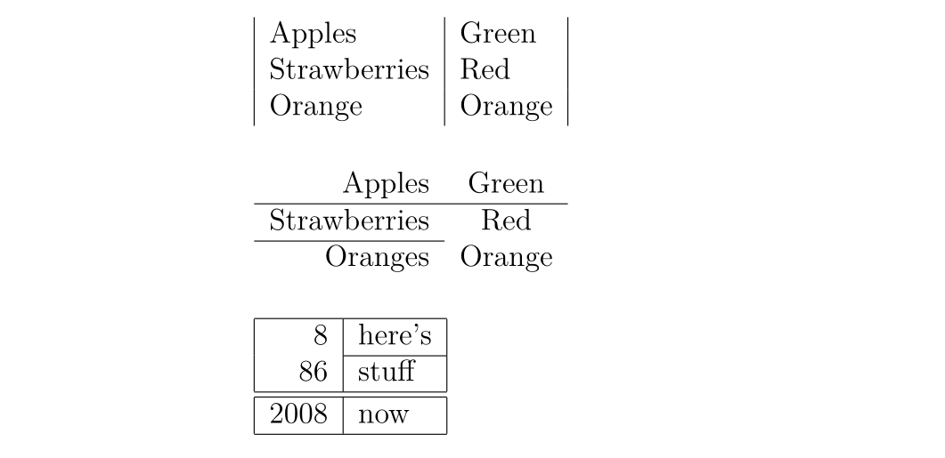
Finally, end the table with \end{tabular}. Here are some examples:
\begin{tabular}{|l|l|}
  Apples       & Green  \\
  Strawberries & Red    \\
  Orange       & Orange \\
\end{tabular}

\begin{tabular}{rc}
  Apples              & Green  \\
  \hline
  Strawberries        & Red    \\
  \cline{1-1} Oranges & Orange \\
\end{tabular}

\begin{tabular}{|r|l|}
  \hline
  8              & here's \\
  \cline{2-2} 86 & stuff  \\
  \hline
  \hline
  2008           & now    \\
  \hline
\end{tabular}
The result is as follows:
Practice
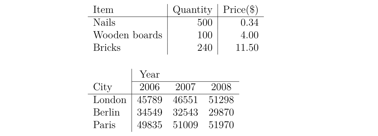
Try to draw the following table:
Figures
This section introduces how to insert figures into LaTeX documents. Here we need to load the graphicx package. Images should be PDF, PNG, JPEG, or GIF files. The following code inserts an image named myimage:
\begin{figure}[h]
  \centering
  \includegraphics[width=1\textwidth]{myimage}
  \caption{Here is my image}
  \label{image-myimage}
\end{figure}
[h] is a placement option; h means to place the figure approximately here, if it fits. Other options are available: t places it at the top of the page; b places it at the bottom; p starts a new page for the figure. You can also add a ! option to force placement at the specified position (although the resulting layout may not be ideal).
\centering places the image at the center of the page. Without this command, it is left-aligned by default. Using it works well because the figure caption is centered as well.
The \includegraphics{...} command automatically places an image in your document; the image file should be in the same directory as the TeX file.
[width=1\textwidth] is an optional argument specifying the image width—the same as the text width. The width can also be given in centimeters. You can use [scale=0.5] to scale the image down (the example reduces it by half).
\caption{...} defines the figure caption. If it is used, LaTeX adds a numbered label beginning with “Figure” to the figure. You can use \listoffigures to generate a list of figures.
\label{...} creates a label that can be referenced.
Practice
Add \usepackage{graphicx} to the preamble of your document. Find an image and place it in your LaTeX course folder. Enter the following where you want to add the image:
\begin{figure}[h!]
  \centering
  \includegraphics[width=1\textwidth]{ImageFilename}
  \caption{My test image}
\end{figure}
Replace ImageFilename with the name of your file, without the extension. If the filename contains spaces, enclose it in double quotes, such as "screen 20".
Compile and check the file.
Equations
One of the main reasons to use LaTeX is that it makes typesetting formulas convenient. We use math mode to typeset formulas.
Inserting equations
You can use a pair of $ characters to enable math mode, which can be used to write inline mathematical formulas. For example, $1+2=3$ produces .
For a displayed formula, you can use $$...$$ (we now recommend \[...\] because the former can introduce undesirable spacing). For example, $$1+2=3$$ produces
For a numbered formula, use \begin{equation}...\end{equation}. For example:
\begin{equation}
  1+2=3
\end{equation}
The result is:

The number 6 is the section number and appears only when sections are configured in the document, for example in a report document.
Use \begin{eqnarray}...\end{eqnarray} to write a group of numbered formulas. For example:
\begin{eqnarray}
  a & = & b + c \\
  & = & y - z
\end{eqnarray}
The result is:

To write unnumbered formulas, add the * character after the environment name, as in {equation*} and {eqnarray*}.
Warning
When using eqnarray, you may find that the spacing around the equals signs is too large.
You can use the amsmath environment from the align package:
\usepackage{amsmath}
...
\begin{align}
  a & = b + c \\
    & = y - z
\end{align}
Or use the aligned environment in a displayed formula. Adding an asterisk after their names makes the formulas unnumbered.
See “4.4 Multi-line formulas” in the first resource under Further reading.
Mathematical symbols
Although some basic symbols can be typed directly, most special symbols need to be displayed with commands.
This book is only an introductory tutorial on using mathematical symbols. The mathematical symbols chapter of the LaTeX Wikibook is another, better, and more complete tutorial. Go there if you want to learn more about mathematical symbols. If you want to find a particular symbol, you can use Detexify, which can recognize handwritten characters.
Superscripts and subscripts
Superscripts (Powers) are written with ^; for example, $n^2$ produces .
Subscripts (Indices) are written with _; for example, $2_a$ produces .
If a superscript or subscript contains multiple characters, enclose it in braces. For example, $b_{a-2}$ produces .
Fractions
Fractions are inserted with the \frac{numerator}{denominator} command. For example, $$\frac{a}{3}$$ produces
Fractions can be nested. For example, $$\frac{y}{\frac{3}{x}+b}$$ produces
Square roots
Use the \sqrt{...} command to insert a square root. Replace the ellipsis with the expression under the root. If you need to specify the root index, enclose it in square brackets.
For example, $$\sqrt{y^2}$$ produces
and $$\sqrt[x]{y^2}$$ produces
Sums and integrals
Use \sum and \int to insert sums and integrals. For both symbols, use ^ for the upper limit and _ for the lower limit.
$$\sum_{x=1}^5 y^z$$ produces
and $$\int_a^b f(x)$$ produces
Greek letters
A Greek letter can be written with a backslash followed by the name of the Greek letter. The capitalization of the first letter of the name determines the form of the Greek letter. For example:
$\alpha$=$\beta$=$\delta, \Delta$=$\pi, \Pi$=$\sigma, \Sigma$=$\phi, \Phi, \varphi$=$\psi, \Psi$=$\omega, \Omega$=
Practice
Write code to generate the following formula:

If you need help, consult the source code of this page.
Bibliography
Introduction
LaTeX makes it easy to insert bibliographies and tables of contents. This section explains how to use a separate BibTeX file to store references.
BibTeX file types
A BibTeX file contains all the references that you want to cite in your document. Its filename extension is .bib. Its name should be the same as the name of your TeX document. A .bib file is a text file. Enter your references in the following format:
@article{
    Birdetal2001,
    Author = {Bird, R. B. and Smith, E. A. and Bird, D. W.},
    Title = {The hunting handicap: costly signaling in human foraging strategies},
    Journal = {Behavioral Ecology and Sociobiology},
    Volume = {50},
    Pages = {9-19},
    Year = {2001}
}
Each reference first declares its reference type. The example uses @article; other types include @book, @incollection for citing a chapter in a book, and @inproceedings for citing a conference paper. More supported types can be found here.
The braces that follow first contain a citation key. The citation keys of the references you cite must be distinct. You can define the key string yourself, but using the first author's name together with the year is a clear choice.
The next several lines contain information about the reference, in the following format:
Field name = {field contents},
You can use LaTeX commands to produce special text effects. For example, italics can be written with \emph{Rattus norvegicus}.
For letters that should remain uppercase, enclose them in braces. BibTeX automatically changes every uppercase letter except the first one in a title to lowercase. For example, Dispersal in the contemporary United States produces , whereas Dispersal in the contemporary {U}nited {S}tates produces .
You can write BibTeX files by hand or use software to generate them.
Inserting the bibliography
Use the following commands to insert a bibliography at the current location in the document:
\bibliographystyle{plain}
\bibliography{references}
The references are written in references.bib.
Citing references
Use \cite{citationkey} to insert a citation where you want to cite a reference. If you do not want to insert a citation in the body but do want the reference to appear in the bibliography, use the \nocite{citationkey} command.
To include page information in a citation, use square brackets: \cite[p. 215]{citationkay}.
To cite multiple references, separate them with commas: \cite{citation01,citation02,citation03}.
Citation styles
Numeric citations
LaTeX includes several formats for inline numeric citations:
Plain uses numbers in square brackets, such as . The bibliography is ordered alphabetically by first author. Each author's full name is used.
Abbrv is the same as plain, but authors' names are abbreviated.
Unsrt is the same as plain, but the bibliography is ordered by the order in which references are cited in the text.
Alpha is like plain, but the citation label combines the author's name and year rather than using a number, such as .
Author–date citations
If you want author–date citations, use the natbib package. It uses the \citep{...} command to generate a citation in square brackets, such as , and \citet{...} to generate a citation with only the year in square brackets, such as . See here for more usage information.
The Natbib package also has three formats: plainnat, abbrvnat, and unsrtnat. They have the same effects as plain, abbrv, and unsrt, respectively.
Other citation styles
If you need a different style, create a format file (a .bst file) in the same folder. When citing this style, use its filename in the \bibliographystyle{...} command.
Practice
Create a BibTeX file with the same name in the same folder, and enter the reference information in the correct format. Switch to the TeX document and use the \cite, \bibliographystyle, and \bibliograph commands to cite the references. Compile the TeX file. Switch to the BibTeX file and compile it (click the Typeset button). Switch back to the TeX file, compile it twice, and check the PDF document.
Further reading
-
A (not very) short introduction to LATEX 2ε https://github.com/CTeX-org/lshort-zh-cn/releases/download/v6.02/lshort-zh-cn.pdf or “Understanding LaTeX 2ε in 112 minutes”.
-
LaTeX Project http://www.latex-project.org/ Official website - has links to documentation, information about installing LATEX on your own computer, and information about where to look for help.
-
LaTeX Wikibook http://en.wikibooks.org/wiki/LaTeX/ Comprehensive and clearly written, although still a work in progress. A downloadable PDF is also available.
-
Comparison of TeX Editors on Wikipedia http://en.wikipedia.org/wiki/Comparison_of_TeX_editors Information to help you choose which LaTeX editor to install on your computer.
-
TeX Live http://www.tug.org/texlive/ "An easy way to get up and running with the TeX document production system". Available for Unix and Windows (with a link to MacTeX for MacOSX users). Includes the TeXworks editor.
-
Workbook Source Files http://edin.ac/17EQPM1 Download the .tex file and other files needed to compile this workbook.
This article was translated from http://www.docs.is.ed.ac.uk/skills/documents/3722/3722-2014.pdf, with some modifications based on other references.