Definition
(Do you remember these definitions? Before reading the following content, make sure you understand the basics in Graph concepts.)
- Path
- Shortest path
- Shortest paths in directed and undirected graphs
- Single-source shortest paths and shortest paths between every pair of vertices
Notation
For convenience, we first define the notation used below.
- is the number of vertices in the graph, and is the number of edges;
- is the source vertex of the shortest paths;
- is the actual shortest-path length from to ;
- is the estimated shortest-path length from to . At all times, . In particular, when a shortest-path algorithm terminates, we should have .
- is the weight of edge .
Properties
In a graph with positive edge weights, a shortest path between any two vertices does not visit a vertex more than once.
In a graph with positive edge weights, a shortest path between any two vertices does not traverse an edge more than once.
In a graph with positive edge weights, any shortest path between two vertices contains at most vertices and at most edges.
Floyd–Warshall algorithm
The Floyd–Warshall algorithm finds shortest paths between every pair of vertices.
Its complexity is relatively high, but its constant factor is small and it is easy to implement (there are only three for loops).
It applies to any graph, directed or undirected and with positive or negative edge weights, provided that the shortest paths exist (that is, there is no negative cycle).
Implementation
Define an array f[k][x][y] as the shortest-path length from vertex to vertex when only vertices through may be used as intermediate vertices (that is, paths in the subgraph ; note that and need not belong to this subgraph).
Clearly, f[n][x][y] is the shortest-path length from to , because is the whole vertex set , so the shortest path it represents is the desired one.
Now consider how to compute the values of the f array.
f[0][x][y] is the edge weight between and , or , or (f[0][x][y] should be when and are directly connected, and when the value is zero because the distance to itself is zero; when and are not directly connected, the value is ).
f[k][x][y] = min(f[k-1][x][y], f[k-1][x][k]+f[k-1][k][y]) (f[k-1][x][y] is the shortest path that does not pass through , while f[k-1][x][k]+f[k-1][k][y] is the shortest path that does pass through ).
Both lines above are immediate, so this approach uses space. We increase the problem size in order ( from to ) and determine the shortest path between every pair under the current problem size.
C++
for (k = 1; k <= n; k++) {
  for (x = 1; x <= n; x++) {
    for (y = 1; y <= n; y++) {
      f[k][x][y] = min(f[k - 1][x][y], f[k - 1][x][k] + f[k - 1][k][y]);
    }
  }
}
Python
for k in range(1, n + 1):
    for x in range(1, n + 1):
        for y in range(1, n + 1):
            f[k][x][y] = min(f[k - 1][x][y], f[k - 1][x][k] + f[k - 1][k][y])
Because the first dimension does not affect the result, we can omit it and write f[x][y] = min(f[x][y], f[x][k]+f[k][y]) directly.
Proof that the first dimension does not affect the result
For a fixed k, when updating f[k][x][y], the referenced elements always come from row k and column k of the f[k-1] array. For this fixed k, updating f[k][k][y] or f[k][x][k] never changes a value: by f[k][k][y] = min(f[k-1][k][y], f[k-1][k][k]+f[k-1][k][y]), f[k-1][k][k] is 0, so the result is always f[k-1][k][y]; the proof for f[k][x][k] is analogous.
Therefore, after omitting the first dimension, none of the values used in an update for a fixed k has been updated during that iteration, so the result is unchanged.
C++
for (k = 1; k <= n; k++) {
  for (x = 1; x <= n; x++) {
    for (y = 1; y <= n; y++) {
      f[x][y] = min(f[x][y], f[x][k] + f[k][y]);
    }
  }
}
Python
for k in range(1, n + 1):
    for x in range(1, n + 1):
        for y in range(1, n + 1):
            f[x][y] = min(f[x][y], f[x][k] + f[k][y])
Thus the time complexity is and the space complexity is .
Applications
Given an undirected graph with positive edge weights, find a cycle with minimum total weight.
Such a cycle must be simple.
Consider how this cycle is formed.
Let be the vertex with the largest index on the cycle.
f[u-1][x][y] together with edges and forms the cycle.
Enumerate during Floyd–Warshall and compute the minimum of these sums.
The time complexity is .
See the minimum cycle section for more details.
Given whether every pair of vertices in a directed graph is connected by an edge, determine whether every pair of vertices is connected.
This is the problem of finding the transitive closure of a graph.
We only need to add vertices one by one following the Floyd–Warshall process.
Here the edge weights become , and is replaced by the OR operation.
Applying a further bitset optimization reduces the complexity to .
// std::bitset<SIZE> f[SIZE];
for (k = 1; k <= n; k++)
  for (i = 1; i <= n; i++)
    if (f[i][k]) f[i] = f[i] | f[k];
Bellman–Ford algorithm
Bellman–Ford is a shortest-path algorithm based on relaxation. It can find shortest paths in graphs with negative edge weights and determine when a shortest path does not exist.
In the domestic OI community, the algorithm known as SPFA is one implementation of Bellman–Ford.
Process
First, let us introduce the relaxation operation used by Bellman–Ford (Dijkstra also uses relaxation).
For an edge , relaxation is represented by the formula .
The meaning is straightforward: try to update the shortest-path length using the path , where the path is a shortest path; if this path is better, update vertex .
Bellman–Ford repeatedly attempts to relax every edge in the graph. Each round attempts one relaxation on every edge; when a round makes no successful relaxation, the algorithm stops.
Each round takes time, so how many rounds can there be at most?
When shortest paths exist, each relaxation increases the number of edges on the shortest path by at least , while a shortest path has at most edges. Therefore the algorithm performs at most rounds of relaxation, and the total time complexity is .
There is another possibility: if starting from we reach a negative cycle, relaxation continues indefinitely. The argument above shows that, when shortest paths exist, at most rounds are needed. Therefore, if an edge can still be relaxed in round , then a negative cycle is reachable from .
A common misconception when detecting negative cycles
When Bellman–Ford is run with as its source and does not report a negative cycle, this only means that no negative cycle is reachable from ; it does not mean that the graph contains no negative cycle.
To determine whether the whole graph contains a negative cycle, the most rigorous approach is to add a super-source with a zero-weight edge to every vertex, then run Bellman–Ford from the super-source.
Implementation
Reference implementation
C++
struct Edge {
  int u, v, w;
};

vector<Edge> edge;

int dis[MAXN], u, v, w;
constexpr int INF = 0x3f3f3f3f;

bool bellmanford(int n, int s) {
  memset(dis, 0x3f, (n + 1) * sizeof(int));
  dis[s] = 0;
  bool flag = false;  // Whether this round performed a relaxation
  for (int i = 1; i <= n; i++) {
    flag = false;
    for (int j = 0; j < edge.size(); j++) {
      u = edge[j].u, v = edge[j].v, w = edge[j].w;
      if (dis[u] == INF) continue;
      // Infinity remains infinity after adding or subtracting a constant
      // Therefore an edge from a vertex whose distance is INF cannot be relaxed
      if (dis[v] > dis[u] + w) {
        dis[v] = dis[u] + w;
        flag = true;
      }
    }
    // Stop when no edge can be relaxed
    if (!flag) {
      break;
    }
  }
  // If relaxation is still possible in round n, s can reach a negative cycle
  return flag;
}
Python
class Edge:
    def __init__(self, u=0, v=0, w=0):
        self.u = u
        self.v = v
        self.w = w


INF = 0x3F3F3F3F
edge = []


def bellmanford(n, s):
    dis = [INF] * (n + 1)
    dis[s] = 0
    for i in range(1, n + 1):
        flag = False
        for e in edge:
            u, v, w = e.u, e.v, e.w
            if dis[u] == INF:
                continue
            # Adding or subtracting a constant from infinity still gives infinity
            # Therefore, an edge leaving a vertex whose shortest-path length is INF cannot be relaxed
            if dis[v] > dis[u] + w:
                dis[v] = dis[u] + w
                flag = True
        # Stop the algorithm when no edge can be relaxed
        if not flag:
            break
    # If relaxation is still possible in the nth iteration, s can reach a negative cycle
    return flag
Queue optimization: SPFA
That is, the Shortest Path Faster Algorithm.
In many cases, we do not need so many unnecessary relaxations.
Clearly, only edges incident to vertices relaxed in the previous round can possibly cause the next relaxation.
We can therefore maintain a queue of “vertices that may cause a relaxation” and visit only the necessary edges.
SPFA can also determine whether vertex can reach a negative cycle: record the number of edges on the shortest path, and if it reaches at least , then can reach a negative cycle.
Implementation
C++
struct edge {
  int v, w;
};

vector<edge> e[MAXN];
int dis[MAXN], cnt[MAXN], vis[MAXN];
queue<int> q;

bool spfa(int n, int s) {
  memset(dis, 0x3f, (n + 1) * sizeof(int));
  dis[s] = 0, vis[s] = 1;
  q.push(s);
  while (!q.empty()) {
    int u = q.front();
    q.pop(), vis[u] = 0;
    for (auto ed : e[u]) {
      int v = ed.v, w = ed.w;
      if (dis[v] > dis[u] + w) {
        dis[v] = dis[u] + w;
        cnt[v] = cnt[u] + 1;  // Number of edges on the shortest path
        if (cnt[v] >= n) return false;
        // Without a negative cycle, a shortest path uses at most n - 1 edges
        // More than n edges therefore imply a negative cycle
        if (!vis[v]) q.push(v), vis[v] = 1;
      }
    }
  }
  return true;
}
Python
from collections import deque


class Edge:
    def __init__(self, v=0, w=0):
        self.v = v
        self.w = w


e = [[Edge() for i in range(MAXN)] for j in range(MAXN)]
INF = 0x3F3F3F3F


def spfa(n, s):
    dis = [INF] * (n + 1)
    cnt = [0] * (n + 1)
    vis = [False] * (n + 1)
    q = deque()

    dis[s] = 0
    vis[s] = True
    q.append(s)
    while q:
        u = q.popleft()
        vis[u] = False
        for ed in e[u]:
            v, w = ed.v, ed.w
            if dis[v] > dis[u] + w:
                dis[v] = dis[u] + w
                cnt[v] = cnt[u] + 1  # Record the number of edges on the shortest path
                if cnt[v] >= n:
                    return False
                # Without a negative cycle, a shortest path uses at most n - 1 edges
                # Therefore, using more than n edges indicates that a negative cycle was traversed
                if not vis[v]:
                    q.append(v)
                    vis[v] = True
Although SPFA is fast in most cases, its worst-case time complexity is , and constructing cases that force this complexity is not difficult. Use it cautiously in contests: when there are no negative edges, Dijkstra is preferable; when negative edges exist but the graph has no special properties, if SPFA is part of the intended solution, the problem should not provide limits that Bellman–Ford cannot handle.
Other Bellman–Ford optimizations
Besides queue optimization (SPFA), Bellman–Ford has other forms of optimization. These can be effective on some graphs, but their worst-case complexity may be exponential on certain special graphs.
- Heap optimization: replace the queue with a heap. Unlike Dijkstra, a vertex may enter the queue multiple times. On graphs with negative edges, the complexity can be forced to exponential.
- Stack optimization: replace the queue with a stack (turning the original BFS process into DFS). It may be more efficient when searching for negative cycles, but its worst-case time complexity remains exponential.
- LLL optimization: replace the ordinary queue with a deque. Compare the distance of the newly enqueued vertex with the average distance in the deque; if it is larger, insert it at the back, otherwise at the front.
- SLF optimization: replace the ordinary queue with a deque. Compare the distance of the newly enqueued vertex with the front vertex; if it is larger, insert it at the back, otherwise at the front.
- D´Esopo–Pape algorithm: replace the ordinary queue with a deque. If a vertex has never been enqueued, insert it at the back; otherwise insert it at the front.
More optimizations and ways to hack these optimizations can be found in fstqwq's Zhihu answer.
Dijkstra algorithm
The Dijkstra algorithm (/ˈdikstrɑ/ or /ˈdɛikstrɑ/) was discovered by Dutch computer scientist E. W. Dijkstra in 1956 and published in 1959. It is a single-source shortest-path algorithm for graphs with nonnegative edge weights.
Process
Partition the vertices into two sets: , the set whose shortest-path lengths have been determined, and , the set whose shortest-path lengths have not been determined. Initially every vertex belongs to .
Initialize and set to for every other vertex.
Then repeatedly perform these operations:
- Select from a vertex with the smallest shortest-path length and move it to .
- Relax all outgoing edges of the vertices just added to .
When becomes empty, the algorithm terminates.
Time complexity
In the naive implementation, after each operation 2, scan directly to find the vertex with the smallest shortest-path length. Operation 2 takes in total, operation 1 takes in total, and the overall complexity is .
A heap can optimize this process: after successfully relaxing an edge , insert into the heap (or perform Decrease-key if is already there), so operation 1 simply takes the heap top. There are Decrease-key operations and pop operations. Different heaps give different complexities; see the heap page. The best complexity achievable with heap optimization is , as with Fibonacci heaps.
In particular, a priority queue can be used. It does not support Decrease-key, but each relaxation can insert the vertex again; when a vertex is popped, check whether it has already been relaxed and skip it if so. The complexity is , with the advantage of simpler implementation.
This heap can also be implemented with a segment tree, with complexity . In some special iterative segment-tree implementations, its constant factor is smaller than that of a heap. A segment tree also supports more operations, and is the only viable structure for some special graph problems.
In a sparse graph, , so heap-optimized Dijkstra is substantially more efficient; in a dense graph, , so the naive implementation is better.
Correctness proof
We prove the correctness of Dijkstra1 by mathematical induction under the assumption that all edge weights are nonnegative.
In short, we must prove that when operation 1 extracts vertex , its shortest path has already been determined, namely .
Initially , so the claim holds.
We now use contradiction.
Let be the first vertex in the algorithm that, when added to , fails to satisfy . Since necessarily satisfies and is necessarily the first vertex added to , before is added to , we have . If no path from to exists, then , contradicting the assumption.
Thus there is a path , where is the first vertex in along the path from , and is the predecessor of (clearly ). Note that or is possible, so or may be an empty path.
All vertices added before satisfy , so when is added to , . Edge is then relaxed, which proves that when is added to , we have .
We now prove . Along the path , all edge weights are nonnegative, so . Hence . However, when vertex is extracted from in operation 1, vertex has not yet been extracted from , so . Thus , contradicting the assumption . The assumption is false.
Therefore every vertex extracted by operation 1 already has its shortest path determined. The proposition follows.
The key inequality in this proof depends on all edge weights being nonnegative. If the graph contains a negative edge, this inequality need not hold, so Dijkstra's correctness is no longer guaranteed and the algorithm may produce an incorrect result.
Implementation
Here we give both an brute-force implementation and an priority-queue implementation.
Naive implementation
C++
struct edge {
  int v, w;
};

vector<edge> e[MAXN];
int dis[MAXN], vis[MAXN];

void dijkstra(int n, int s) {
  memset(dis, 0x3f, (n + 1) * sizeof(int));
  dis[s] = 0;
  for (int i = 1; i <= n; i++) {
    int u = 0, mind = 0x3f3f3f3f;
    for (int j = 1; j <= n; j++)
      if (!vis[j] && dis[j] < mind) u = j, mind = dis[j];
    vis[u] = true;
    for (auto ed : e[u]) {
      int v = ed.v, w = ed.w;
      if (dis[v] > dis[u] + w) dis[v] = dis[u] + w;
    }
  }
}
Python
class Edge:
    def __init(self, v=0, w=0):
        self.v = v
        self.w = w


e = [[Edge() for i in range(MAXN)] for j in range(MAXN)]
INF = 0x3F3F3F3F


def dijkstra(n, s):
    dis = [INF] * (n + 1)
    vis = [0] * (n + 1)

    dis[s] = 0
    for i in range(1, n + 1):
        u = 0
        mind = INF
        for j in range(1, n + 1):
            if not vis[j] and dis[j] < mind:
                u = j
                mind = dis[j]
        vis[u] = True
        for ed in e[u]:
            v, w = ed.v, ed.w
            if dis[v] > dis[u] + w:
                dis[v] = dis[u] + w
Priority-queue implementation
C++
struct edge {
  int v, w;
};

struct node {
  int dis, u;

  bool operator>(const node& a) const { return dis > a.dis; }
};

vector<edge> e[MAXN];
int dis[MAXN], vis[MAXN];
priority_queue<node, vector<node>, greater<node>> q;

void dijkstra(int n, int s) {
  memset(dis, 0x3f, (n + 1) * sizeof(int));
  memset(vis, 0, (n + 1) * sizeof(int));
  dis[s] = 0;
  q.push({0, s});
  while (!q.empty()) {
    int u = q.top().u;
    q.pop();
    if (vis[u]) continue;
    vis[u] = 1;
    for (auto ed : e[u]) {
      int v = ed.v, w = ed.w;
      if (dis[v] > dis[u] + w) {
        dis[v] = dis[u] + w;
        q.push({dis[v], v});
      }
    }
  }
}
Python
def dijkstra(e, s):
    """
    Input:
    e: adjacency list
    s: source vertex
    Returns:
    dis: shortest-path distance from s to every vertex
    """
    dis = defaultdict(lambda: float("inf"))
    dis[s] = 0
    q = [(0, s)]
    vis = set()
    while q:
        _, u = heapq.heappop(q)
        if u in vis:
            continue
        vis.add(u)
        for v, w in e[u]:
            if dis[v] > dis[u] + w:
                dis[v] = dis[u] + w
                heapq.heappush(q, (dis[v], v))
    return dis
Johnson's all-pairs shortest-path algorithm
Like Floyd–Warshall, Johnson's algorithm finds shortest paths between every pair of vertices in a graph without negative cycles. It was proposed by Donald B. Johnson in 1977.
We can enumerate the source and run Bellman–Ford times, in time, or solve the problem directly with Floyd–Warshall in time.
Heap-optimized Dijkstra has lower single-source complexity than Bellman–Ford. Enumerating the source and running Dijkstra times solves the problem in time (depending on the Dijkstra implementation), which is better than running Bellman–Ford times and also better than Floyd–Warshall on sparse graphs.
However, Dijkstra cannot correctly handle negative edges, so we must preprocess the edges of the original graph so that all edge weights become nonnegative.
An obvious idea is to add the same positive number to every edge weight. If a shortest path in the new graph uses edges, subtracting from its length gives the actual shortest-path length.
But this method is incorrect. Consider the following graph:
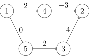
The shortest path from is , with length .
What if we add to the weight of every edge?
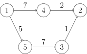
In the new graph, the shortest path from is , which is no longer the actual shortest path.
Johnson's algorithm instead reweights every edge in another way.
Create a virtual vertex (numbered here), and add an edge of weight from it to every other vertex.
Run Bellman–Ford to find the shortest paths from vertex to all other vertices, denoted by .
If there is an edge from to with weight , reset its weight to .
Then run Dijkstra times, once from each vertex, to obtain the shortest paths between every pair.
The initial Bellman–Ford run is not the time bottleneck. With Dijkstra implemented by priority_queue, the time complexity is .
Correctness proof
Why is this reweighting correct?
Before answering that question, let us discuss the physical concept of potential energy.
Potential energies such as gravitational and electric potential energy share one property: the change in potential depends only on the relative positions of the start and end points, not on the path taken between them.
Potential energy also has another property: its absolute value usually depends on where the zero-potential reference is set, but the difference in potential between two points is fixed regardless of that choice.
Now return to the algorithm.
On the reweighted graph, the length of a path from to , namely , is:
After simplification:
No matter which path we take from to , the value of is constant, exactly as the potential-energy property suggests.
For convenience, we call the potential energy of vertex below.
The expression for the length of the shortest path in the new graph has two parts: the first is the sum of the original edge weights along the path, and the second is the potential difference between the two vertices. Since the potential difference between is fixed, the shortest path in the original graph corresponds to the shortest path in the new graph.
This completes half of the correctness proof: after reweighting, the shortest paths in the graph are still the original shortest paths. We must now prove that every edge in the new graph has nonnegative weight, because Dijkstra is guaranteed to be correct on a graph with nonnegative edge weights.
By the triangle inequality, the endpoints of every edge satisfy . Its reweighted weight is . Thus all edge weights in the new graph are nonnegative.
This proves the correctness of Johnson's algorithm.
Comparison of different methods
| Shortest-path algorithm | Floyd–Warshall | Bellman–Ford | Dijkstra | Johnson |
|---|---|---|---|---|
| Shortest-path type | All-pairs shortest paths | Single-source shortest paths | Single-source shortest paths | All-pairs shortest paths |
| Applicable graphs | Any graph | Any graph | Graphs with nonnegative edge weights | Any graph |
| Can detect negative cycles? | Yes | Yes | No | Yes |
| Time complexity |
Note: the Dijkstra implementation used for the complexity entries in the table uses priority_queue.
Outputting the path
Create a pre array and record how each vertex was reached whenever a distance is updated; before the algorithm ends, recursively output the path.
For example, Floyd–Warshall records pre[i][j] = k;, while Bellman–Ford and Dijkstra generally record pre[v] = u.
Special cases
- Shortest paths in a graph whose edge weights are only and : 0-1 BFS;
- Shortest-path problems that allow at most operations such as changing the path cost: shortest paths on layered graphs.
References and notes
Footnotes
-
Introduction to Algorithms, 3rd Chinese edition, China Machine Press, 2013, pp. 384–385. ↩