Dominator Tree

Preface

In 1959, Reese T. Prosser proposed the concept of dominators in a paper on network flows, but did not propose a specific algorithm. It was not until 1969 that Edward S. Lowry and C. W. Medlock first proposed an effective algorithm. The currently most widely used Lengauer–Tarjan algorithm was proposed by Lengauer and Tarjan in 1979 in a paper.

In the OI community, the concept of dominator trees was first introduced in ZJOI2012 Disaster, where it was also called an “extinction tree”. Chen Sunli also introduced this algorithm in a 2020 national training team paper.

Dominator trees are not currently popular in competitive programming, and related exercises are uncommon; however, they are widely used in industry, especially in compiler-related fields.

This article introduces the concept of dominator trees and several ways to compute them.

Dominance relation

In any directed graph, designate an entry node $s$. For a node $u$, if every path from $s$ to $u$ passes through a node $v$, then we say that $v$ dominates $u$, also call $v$ a dominator of $u$, and write $v\ dom\ u$.

Discussing dominance relations for nodes unreachable from $s$ is meaningless. Therefore, unless otherwise specified, this article assumes that $s$ can reach every node in the graph.

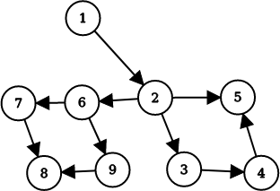
For example, in this directed graph, $2$ is dominated by $1$, $3$ is dominated by $1, 2$, 4 is dominated by $1, 2, 3$, 5 is dominated by $1, 2$, etc.

Lemmas

In the lemmas below, assume $u, v, w\ne s$.

Lemma 1: $s$ is a dominator of every node; every node is a dominator of itself.

Proof: Every path from $s$ to $u$ must pass through both $s$ and $u$.

Lemma 2: The dominance relation obtained by considering only simple paths is the same as the relation obtained by considering all paths.

Proof: For a nonsimple path, let $S$ be the set of all nodes visited between two visits to a node. Deleting the nodes in $S$ makes each nonsimple path correspond to a simple path.

A node in $S$ that lies on the nonsimple path but not on the simple path cannot be a dominator, because there is at least one simple path from $s$ to $u$ that does not include it. Nodes on both the simple and nonsimple paths only need to be considered on the simple path.

In summary, deleting nonsimple paths does not affect the dominance relation.

Lemma 3: If $u$ $dom$ $v$, and $v$ $dom$ $w$, then $u$ $dom$ $w$.

Proof: Every path through $w$ must pass through $v$, and every path through $v$ must pass through $u$. Therefore, every path through $w$ must pass through $u$, namely $u \ dom \ w$.

Lemma 4: If $u \ dom \ v$ and $v \ dom\ u$, then $u=v$.

Proof: Suppose $u \ne v$. Then every path reaching $v$ has already reached $u$, while every path reaching $u$ has already reached $v$, a contradiction.

Lemma 5: If $u \ne v \ne w$, $u \ dom \ w$, and $v \ dom \ w$, then either $u \ dom \ v$ or $v \ dom \ u$.

Proof: Consider a path $s \rightarrow \dots \rightarrow u \rightarrow \dots \rightarrow v \rightarrow \dots \rightarrow w$. If $u$ and $v$ do not dominate one another, there must be a path that does not pass through $u$, from $s$ to $v$, namely $s \rightarrow \dots \rightarrow v \rightarrow \dots \rightarrow w$, contradicting $u\ dom\ w$.

Computing dominance relations

Node-deletion method

A conclusion equivalent to the definition is the following: if deleting a node from the graph makes some nodes unreachable, then the deleted node dominates those nodes that became unreachable.

Therefore, we can simply delete each node in turn and run dfs; the code complexity is $O(n^3)$. The core code is given below.

// Suppose the graph has n nodes, with starting node s = 1
std::bitset<N> vis;
std::vector<int> edge[N];
std::vector<int> dom[N];

void dfs(int u, int del) {
  vis[u] = true;
  for (int v : edge[u]) {
    if (v == del or vis[v]) {
      continue;
    }
    dfs(v, del);
  }
}

void getdom() {
  for (int i = 2; i <= n; ++i) {
    vis.reset();
    dfs(1, i);
    for (int j = 1; j <= n; ++j) {
      if (!vis[j]) {
        dom[j].push_back(i);
      }
    }
  }
}

Data-flow iteration method

The data-flow iteration method is also an uncommon topic in OI, so we first give a brief introduction.

Data-flow analysis is a concept in compiler theory used to analyze how data flows along program-execution paths. Data-flow iteration writes equations at the nodes of a program's flow graph and repeatedly solves them to obtain data-flow values at certain program points. Here, we regard the directed graph as a program flow graph.

The equation in this problem is:

Here, $pre(u)$ is the set of predecessor nodes of $u$. This equation follows from Lemma 3.

In plain language, the set of dominators of a node is the intersection of the dominator sets of all its predecessors, together with the node itself. Repeatedly iterate the dominator set at each node according to this equation until the answer no longer changes.

To improve efficiency, we hope that in each iteration, as many predecessors as possible of the node currently being iterated have already completed that iteration. Therefore, we use depth-first ordering to obtain the reverse postorder of the graph and iterate in that order.

Here is a reference implementation of the core code. The predecessor set of each node and the reverse postorder of the graph must be precomputed; these are not the main topics of this article, so their implementations are omitted.

std::vector<int> pre[N];  // predecessors of each node
std::vector<int> ord;     // reverse postorder of the graph
std::bitset<N> dom[N];
std::vector<int> Dom[N];

void getdom() {
  dom[1][1] = true;
  flag = true;
  while (flag) {
    flag = false;
    for (int u : ord) {
      std::bitset<N> tmp;
      tmp[u] = true;
      for (int v : pre[u]) {
        tmp &= dom[v];
      }
      if (tmp != dom[u]) {
        dom[u] = tmp;
        flag = true;
      }
    }
  }
  for (int i = 2; i <= n; ++i) {
    for (int j = 1; j <= n; ++j) {
      if (dom[i][j]) {
        Dom[i].push_back(j);
      }
    }
  }
}

It is not difficult to see that the complexity of the algorithm above is $O(n^2)$.

Dominator tree

In the previous section, we saw that every node other than $s$ has at least two dominators: $s$ and itself.

Among the dominators of any node $u$, call the node $v$ other than itself that is closest to it the immediate dominator of $u$, denoted by $idom(u) = v$. Clearly, every node has a unique immediate dominator except $s$, which has none.

For every node other than $s$, $u$, add an edge from $idom(u)$ to $u$; this forms a directed graph with $n$ nodes and $n - 1$ edges. By Lemmas 3 and 4, the dominance relation cannot form a cycle, so these edges cannot form a cycle either. Thus the graph is in fact a tree. We call this tree the dominator tree of the original graph.

Computing the dominator tree

Computing from dom

Consider a dominator set $\{s_1, s_2, \dots, s_k\}$ of a node. There must be a path $s \rightarrow \dots \rightarrow s_1 \rightarrow \dots \rightarrow s_2 \rightarrow \dots \rightarrow \dots \rightarrow s_k \rightarrow\dots \rightarrow u$. Clearly, the immediate dominator of $u$ is $s_k$. Thus, the definition of an immediate dominator is equivalent to:

For a node $u$ with dominator set $S$, if $v \in S$ satisfies $\forall w \in S\setminus\{u,v\}, w\ dom \ v$, then $idom(u)=v$.

Therefore, after obtaining the dominator set of every node using the algorithm described above, we can easily find the immediate dominator of every node according to this definition and construct the dominator tree. Reference code is given below.

std::bitset<N> dom[N];
std::vector<int> Dom[N];
int idom[N];

void getidom() {
  for (int u = 2; u <= n; ++u) {
    for (int v : Dom[u]) {
      std::bitset<N> tmp = (dom[v] & dom[u]) ^ dom[u];
      if (tmp.count() == 1 and tmp[u]) {
        idom[u] = v;
        break;
      }
    }
  }
  for (int u = 2; u <= n; ++u) {
    e[idom[u]].push_back(u);
  }
}

Special case on a tree

Clearly, the dominator tree of a tree-shaped graph is the graph itself.

Special case on a DAG

A DAG has a useful property: when solving in topological order, a solution found earlier does not affect later solutions. We can use this property to compute the dominator tree of a DAG efficiently.

Lemma 6: In a directed graph, $v\ dom\ u$ if and only if $\forall w \in pre(u), v\ dom \ w$.

Proof: First prove sufficiency. Every path from $s$ to $u$ must pass through a node $w \in pre(u)$, and $v$ dominates this node. Therefore, every path from $s$ to $u$ must pass through $v$, giving $v \ dom \ u$.

Now for necessity. If $\exists w\in pre(u)$ and $v$ does not dominate $w$, there must be a path not passing through $v$, $s \rightarrow \cdots \rightarrow w \rightarrow \cdots \rightarrow u$, so $v$ does not dominate $u$.

We see that the dominators of $u$ are common ancestors of all its predecessor nodes in the dominator tree. Therefore, the immediate dominator of $u$ is the LCA of all predecessor nodes. Using binary lifting to solve LCA supports adding one node at a time, so the algorithm above is clearly feasible.

Reference implementation:

std::stack<int> sta;
std::vector<int> e[N], g[N], tree[N];  // g is the reverse graph; tree is the dominator tree
int n, s, in[N], tpn[N], dep[N], idom[N];  // n is the total number of nodes, s is the starting node, and in is the indegree
int fth[N][17];

void topo(int s) {
  sta.push(s);
  while (!sta.empty()) {
    int u = sta.top();
    sta.pop();
    tpn[++tot] = u;
    for (int v : e[u]) {
      --in[v];
      if (!in[v]) {
        sta.push(v);
      }
    }
  }
}

int lca(int u, int v) {
  if (dep[u] < dep[v]) {
    std::swap(u, v);
  }
  for (int i = 15; i >= 0; --i) {
    if (dep[fth[u][i]] >= dep[v]) {
      u = fth[u][i];
    }
  }
  if (u == v) {
    return u;
  }
  for (int i = 15; i >= 0; --i) {
    if (fth[u][i] != fth[v][i]) {
      u = fth[u][i];
      v = fth[v][i];
    }
  }
  return fth[u][0];
}

void build() {
  topo(s);
  for (int i = 1; i <= n; ++i)
    for (int j = 0; j <= 15; ++j) fth[i][j] = s;
  for (int i = 1; i <= n; ++i) {
    int u = tpn[i];
    if (g[u].size()) {
      int v = g[u][0];
      for (int j = 1, q = g[u].size(); j < q; ++j) {
        v = lca(v, g[u][j]);
      }
      tree[v].push_back(u);
      fth[u][0] = v;
      dep[u] = dep[v] + 1;
      for (int i = 1; i <= 15; ++i) {
        fth[u][i] = fth[fth[u][i - 1]][i - 1];
      }
    }
  }
}

Lengauer–Tarjan Algorithm

The Lengauer–Tarjan algorithm is one of the best-known algorithms for computing dominator trees; it can compute the dominator tree of a directed graph in $O(n\alpha(n, m))$ time. This algorithm introduces the concept of semidominators and uses semidominators to help compute immediate dominators.

Conventions

First, starting from $s$, run dfs on this directed graph; the visited vertices and edges form a tree $T$. We call the traversed edges tree edges and the others nontree edges; let $dfn(u)$ denote the index at which vertex $u$ is visited; define $u<v$ if and only if $dfn(u) < dfn(v)$.

Semidominators

The semidominator of a vertex $u$ is the smallest vertex among those for which there is a path starting from a vertex $v$ such that every vertex on the path other than $u, v$ is greater than $u$. Formally, the semidominator of $u$ is written $sdom(u)$:

$sdom(u) = \min(v|\exists v=v_0 \rightarrow v_1 \rightarrow\dots \rightarrow v_k = u, \forall 1\le i\le k - 1, v_i > u)$

We observe that semidominators have several useful properties:

Lemma 7: For any vertex $u$, $sdom(u) < u$.

Proof: By the definition, it is easy to see that $u$'s parent in $T$, $fa(u)$, also satisfies the conditions for being a semidominator, and $fa(u) < u$; therefore, no vertex greater than $u$ can be its semidominator.

Lemma 8: For any vertex $u$, $idom(u)$ is an ancestor in $T$.

Proof: In $T$, the path from $s$ to $u$ corresponds to a path in the original graph, so $idom(u)$ must lie on this path.

Lemma 9: For any vertex $u$, $sdom(u)$ is an ancestor in $T$.

Proof: Assume that $sdom(u)$ is not an ancestor of $u$. Then $sdom(u)$ cannot have an edge to any vertex whose $\mathrm{dfs}$ order is greater than or equal to that of $u$ (otherwise that vertex should lie in the subtree of $sdom(u)$ rather than in another subtree), a contradiction.

Lemma 10: For any vertex $u$, $idom(u)$ is an ancestor of $sdom(u)$.

Proof: Consider a path that goes from $s$ to $sdom(u)$ and then follows the path in the definition to $u$. By definition, no vertex on the path from $sdom(u)$ to $u$ dominates $u$, so $idom(u)$ must be an ancestor of $sdom(u)$.

Lemma 11: For any vertices $u \ne v$ such that $v$ is an ancestor of $u$, either $v$ is an ancestor of $idom(u)$ or $idom(u)$ is an ancestor of $idom(v)$.

Proof: For any vertex between $v$ and $idom(v)$, call it $w$; by the definition of the immediate dominator, there must be a path avoiding $w$ from $s$ to $idom(v)$ and then to $v$. Therefore, these vertices $w$ are not $idom(u)$, so $idom(u)$ is either a descendant of $v$ or an ancestor of $idom(v)$.

From the lemmas above, we obtain the following theorem:

Theorem 1: The semidominator of a vertex $u$ is the minimum of its predecessors and the semidominators of all ancestors in $T$ greater than $u$ that dominate it. Formally, $sdom(u)=\min(\{v|\exists v \rightarrow u, v < u \} \cup \{sdom(w) | w > u\ and\ \exists w \rightarrow \dots \rightarrow v \rightarrow u \})$.

Proof: Let $x$ equal the right-hand side of the equation above.

First we prove $sdom(u) \le x$. By Lemma 7, this is equivalent to proving that both of the two cases above satisfy the conditions for being a semidominator. The case where $x$ is a predecessor of $u$ is obvious. For the second case, concatenate the path $x=v_0\rightarrow\dots\rightarrow v_j=w$ from the definition of the semidominator with a path in $T$ satisfying $\forall i\in[j, k-1], v_i\ge w > u$, namely $w=v_j \rightarrow\dots\rightarrow v_k=v$, and then with the path $v \rightarrow u$, thereby constructing a path that satisfies the definition of a semidominator.

Next we prove $sdom(u)\ge x$. Consider the path to $u$ specified in the definition of its semidominator, $sdom(u)=v_0\rightarrow v_1 \rightarrow\dots\rightarrow v_k=u$. It is easy to see that $k=1$ and $k > 1$ correspond to the two choices in the definition, respectively. If $k = 1$, there is a directed edge $sdom(u) \rightarrow u$, and the result follows from Lemma 7; if $k>1$, let $j$ be the smallest integer satisfying $j \ge 1$ such that $v_j$ is an ancestor of $v_{k-1}$ in $T$. Since $k$ satisfies the condition above, such a $j$ must exist.

Consider the proof that $v_0 \rightarrow \dots \rightarrow v_j$ is a path satisfying the conditions for being a semidominator of $v_j$, namely that $\forall i \in [1, j), v_i>v_j$. If not, let $i$ be such that $v_i < v_j$, choosing $v_i$ to be the smallest such value. By Lemma 11, we know that $v_i$ is an ancestor of $v_j$, contradicting the definition of $j$. Hence $sdom(v_j)\le sdom(u)$. In conclusion, $sdom(u) \le x$, so $x=sdom(u)$.

By Theorem 1, we can compute the semidominator of every vertex. It is easy to see that the bottleneck in this computation is the second case; we therefore use a weighted disjoint-set union to optimize it, updating the minimum value whenever path compression is performed.

void dfs(int u) {
  dfn[u] = ++dfc;
  pos[dfc] = u;
  for (int i = h[0][u]; i; i = e[i].x) {
    int v = e[i].v;
    if (!dfn[v]) {
      dfs(v);
      fth[v] = u;
    }
  }
}

int find(int x) {
  if (fa[x] == x) {
    return x;
  }
  int tmp = fa[x];
  fa[x] = find(fa[x]);
  if (dfn[sdm[mn[tmp]]] < dfn[sdm[mn[x]]]) {
    mn[x] = mn[tmp];
  }
  return fa[x];
}

void getsdom() {
  dfs(1);
  for (int i = 1; i <= n; ++i) {
    mn[i] = fa[i] = sdm[i] = i;
  }
  for (int i = dfc; i >= 2; --i) {
    int u = pos[i], res = INF;
    for (int j = h[1][u]; j; j = e[j].x) {
      int v = e[j].v;
      if (!dfn[v]) {
        continue;
      }
      find(v);
      if (dfn[v] < dfn[u]) {
        res = std::min(res, dfn[v]);
      } else {
        res = std::min(res, dfn[sdm[mn[v]]]);
      }
    }
    sdm[u] = pos[res];
    fa[u] = fth[u];
  }
}

Computing immediate dominators

Transforming the graph into a DAG

But I still do not know what semidominators are useful for!

On $T$, for every $u$, we add a directed edge $sdom(u) \rightarrow u$. By Lemma 9, the resulting graph $G$ is necessarily a DAG; by Lemma 10, adding these edges does not change the dominance relation, so we have transformed the original graph into a DAG and can solve it using the algorithm above.

Computing through semidominators

Building a pile of graphs is not very elegant!

Theorem 2: For any vertex $u$, if every vertex on the path in $T$ from $sdom(u)$ to $w$, each denoted by $v$, satisfies $sdom(v)\ge sdom(w)$, then $idom(u) =sdom(u)$.

Proof: By Lemma 10, $idom(u)$ is $sdom(u)$ or one of its ancestors, so it suffices to prove $sdom(u) \ dom \ u$.

Consider any path from $s$ to $u$, denoted by $P$; we need to prove that $sdom(u)$ lies on $P$. Let $v$ be the last vertex on $P$ satisfying $v<sdom(u)$. If $v$ does not exist, then $sdom(u)=idom(u) =s$; otherwise, let $w$ be the first vertex on $P$ after $v$ that lies on the path from $sdom(u)$ to $u$ in the DFS tree.

We next prove $sdom(w)\le v <sdom(v)$. Consider in $T$ the path from $v$ to $w$, $v = v_0 \rightarrow \dots v_k = w$. If this is false, there exists $i\in[1, k- 1], v_i < w$. Then there is a $j\in [i, k - 1]$ such that $v_j$ is an ancestor of $w$. From the choice of $v$, we know that $sdom(u)\le v_j$, so $v_j$ also lies on the path from $sdom(u)$ to $u$ in the DFS tree, contradicting the definition of $w$. Therefore $sdom(w)\le v < sdom(v)$; together with the theorem's condition, this gives $y=sdom(u)$, so path $P$ contains $sdom(u)$.

Theorem 3: For any vertex $u$, among all vertices in $T$ on the path from $sdom(u)$ to $u$, let $v$ be the one with the smallest semidominator; then $sdom(v)\le sdom(u)$ and $idom(v) = idom(u)$.

Proof: Since $u$ itself also satisfies the condition for $v$, $sdom(v)\le sdom(u)$.

Since $idom(u)$ is an ancestor of $v$ in $T$, Lemma 11 shows that $idom(u)$ is also an ancestor of $idom(v)$; therefore, it remains only to prove that $idom(v)$ dominates $u$.

Take a path from $s$ to $u$ and call it $P$; it suffices to show that $sdom(u)$ lies on $P$. Let $x$ denote the last vertex on $P$ for which $x<sdom(u)$. If no such $x$ exists, then $sdom(u)=idom(u) =s$; otherwise, let $y$ be the first vertex on $P$ after $x$ lying on the DFS-tree path from $sdom(u)$ to $u$.

By the same reasoning as in the proof of Theorem 2, we obtain $sdom(y) \le x$. By Lemma 10, $sdom(y)\le x<idom(v) \le sdom(v)$. Thus, by the definition of $v$, $y$ cannot be a descendant of $sdom(u)$; moreover, $y$ cannot be both a descendant of $idom(v)$ and an ancestor of $v$, because the path that follows the DFS tree from $s$ to $sdom(y)$, then follows path P to $y$, and finally follows the DFS tree to $v$ does not pass through $idom(v)$, contradicting the definition of a dominator. Therefore $y=idom(v)$, so $P$ contains $idom(v)$.

From the two theorems above, we obtain the relationship between $sdom(u)$ and $idom(u)$.

Let $v$ be the vertex such that $v$ lies between $sdom(u)$ and $u$, chosen so that $sdom(v)$ is the smallest among all such vertices; then:

The code for computing semidominators above only needs a small modification.

struct E {
  int v, x;
} e[MAX * 4];

int h[3][MAX * 2];

int dfc, tot, n, m, u, v;
int fa[MAX], fth[MAX], pos[MAX], mn[MAX], idm[MAX], sdm[MAX], dfn[MAX],
    ans[MAX];

void add(int x, int u, int v) {
  e[++tot] = {v, h[x][u]};
  h[x][u] = tot;
}

void dfs(int u) {
  dfn[u] = ++dfc;
  pos[dfc] = u;
  for (int i = h[0][u]; i; i = e[i].x) {
    int v = e[i].v;
    if (!dfn[v]) {
      dfs(v);
      fth[v] = u;
    }
  }
}

int find(int x) {
  if (fa[x] == x) {
    return x;
  }
  int tmp = fa[x];
  fa[x] = find(fa[x]);
  if (dfn[sdm[mn[tmp]]] < dfn[sdm[mn[x]]]) {
    mn[x] = mn[tmp];
  }
  return fa[x];
}

void tar(int st) {
  dfs(st);
  for (int i = 1; i <= n; ++i) {
    fa[i] = sdm[i] = mn[i] = i;
  }
  for (int i = dfc; i >= 2; --i) {
    int u = pos[i], res = INF;
    for (int j = h[1][u]; j; j = e[j].x) {
      int v = e[j].v;
      if (!dfn[v]) {
        continue;
      }
      find(v);
      if (dfn[v] < dfn[u]) {
        res = std::min(res, dfn[v]);
      } else {
        res = std::min(res, dfn[sdm[mn[v]]]);
      }
    }
    sdm[u] = pos[res];
    fa[u] = fth[u];
    add(2, sdm[u], u);
    u = fth[u];
    for (int j = h[2][u]; j; j = e[j].x) {
      int v = e[j].v;
      find(v);
      if (sdm[mn[v]] == u) {
        idm[v] = u;
      } else {
        idm[v] = mn[v];
      }
    }
    h[2][u] = 0;
  }
  for (int i = 2; i <= dfc; ++i) {
    int u = pos[i];
    if (idm[u] != sdm[u]) {
      idm[u] = idm[idm[u]];
    }
  }
}

Example problems

Luogu P5180 “Template” Dominator Tree

We can compute only the dominance relation, recording how many vertices each vertex dominates, or build the dominator tree and compute the size of every vertex.

The latter approach is implemented below.

#include <iostream>
using std::cin;
using std::cout;
constexpr int MAX = 3e5 + 5;
constexpr int INF = 0x5ffffff;

struct E {
  int v, x;
} e[MAX * 4];

int n, m, u, v, tot, dfc;
int ans[MAX], dfn[MAX], pos[MAX], sdm[MAX], idm[MAX], fa[MAX], mn[MAX],
    fth[MAX];
int h[3][MAX * 2];

void add(int x, int u, int v) {
  e[++tot] = {v, h[x][u]};
  h[x][u] = tot;
}

void dfs(int u) {
  dfn[u] = ++dfc;
  pos[dfc] = u;
  for (int i = h[0][u]; i; i = e[i].x) {
    int v = e[i].v;
    if (!dfn[v]) {
      dfs(v);
      fth[v] = u;
    }
  }
}

int find(int x) {
  if (fa[x] == x) {
    return x;
  }
  int tmp = fa[x];
  fa[x] = find(fa[x]);
  if (dfn[sdm[mn[tmp]]] < dfn[sdm[mn[x]]]) {
    mn[x] = mn[tmp];
  }
  return fa[x];
}

void tar(int st) {
  dfs(st);
  for (int i = 1; i <= n; ++i) {
    mn[i] = fa[i] = sdm[i] = i;
  }
  for (int i = dfc; i >= 2; --i) {
    int u = pos[i], res = INF;
    for (int j = h[1][u]; j; j = e[j].x) {
      int v = e[j].v;
      if (!dfn[v]) {
        continue;
      }
      find(v);
      if (dfn[v] < dfn[u]) {
        res = std::min(res, dfn[v]);
      } else {
        res = std::min(res, dfn[sdm[mn[v]]]);
      }
    }
    sdm[u] = pos[res];
    fa[u] = fth[u];
    add(2, sdm[u], u);
    u = fth[u];
    for (int j = h[2][u]; j; j = e[j].x) {
      int v = e[j].v;
      find(v);
      if (u == sdm[mn[v]]) {
        idm[v] = u;
      } else {
        idm[v] = mn[v];
      }
    }
    h[2][u] = 0;
  }
  for (int i = 2; i <= dfc; ++i) {
    int u = pos[i];
    if (idm[u] != sdm[u]) {
      idm[u] = idm[idm[u]];
    }
  }
  for (int i = dfc; i >= 2; --i) {
    ++ans[pos[i]];
    ans[idm[pos[i]]] += ans[pos[i]];
  }
  ++ans[1];
}

int main() {
  cin >> n >> m;
  for (int i = 1; i <= m; ++i) {
    cin >> u >> v;
    add(0, u, v);
    add(1, v, u);
  }
  tar(1);
  for (int i = 1; i <= n; ++i) {
    cout << ans[i] << ' ';
  }
}

ZJOI2012 Disaster

On a DAG, build the dominator tree and then compute the size of each vertex.

#include <iostream>
#include <stack>
#include <vector>

using std::cin;
using std::cout;
using std::stack;
using std::vector;

constexpr int MAX = 65536;
int n, x, tot;
int d[MAX], w[MAX], siz[MAX], p[MAX], f[MAX][17];
vector<int> e[MAX], g[MAX], h[MAX];
stack<int> s;

void topo() {
  s.push(0);
  for (int i = 1; i <= n; ++i) {
    if (!w[i]) {
      e[0].push_back(i);
      g[i].push_back(0);
      ++w[i];
    }
  }
  while (!s.empty()) {
    int x = s.top();
    s.pop();
    p[++tot] = x;
    for (int i : e[x]) {
      --w[i];
      if (!w[i]) {
        s.push(i);
      }
    }
  }
}

int lca(int u, int v) {
  if (d[u] < d[v]) {
    std::swap(u, v);
  }
  for (int i = 15; i >= 0; --i) {
    if (d[f[u][i]] >= d[v]) {
      u = f[u][i];
    }
  }
  if (u == v) {
    return u;
  }
  for (int i = 15; i >= 0; --i) {
    if (f[u][i] != f[v][i]) {
      u = f[u][i];
      v = f[v][i];
    }
  }
  return f[u][0];
}

void dfs(int x) {
  siz[x] = 1;
  for (int i : h[x]) {
    dfs(i);
    siz[x] += siz[i];
  }
}

void build() {
  for (int i = 2; i <= n + 1; ++i) {
    int x = p[i], y = g[x][0];
    for (int j = 1, q = g[x].size(); j < q; ++j) {
      y = lca(y, g[x][j]);
    }
    h[y].push_back(x);
    d[x] = d[y] + 1;
    f[x][0] = y;
    for (int i = 1; i <= 15; ++i) {
      f[x][i] = f[f[x][i - 1]][i - 1];
    }
  }
}

int main() {
  cin >> n;
  for (int i = 1; i <= n; ++i) {
    while (true) {
      cin >> x;
      if (!x) {
        break;
      }
      e[x].push_back(i);
      g[i].push_back(x);
      ++w[i];
    }
  }
  topo();
  build();
  dfs(0);
  for (int i = 1; i <= n; ++i) {
    cout << siz[i] - 1 << '\n';
  }
  return 0;
}