AIOJ

Introduction

Before reading the following content, be sure to understand the graph-related concepts.

Related reading: Articulation Points and Bridges

Definitions

For more rigorous definitions of articulation points and bridges, see the graph-related concepts.

In a connected undirected graph, for two vertices $u$ and $v$ , if deleting any edge (only one edge may be deleted) cannot make them disconnected, we say that $u$ and $v$ are edge-biconnected.

In a connected undirected graph, for two vertices $u$ and $v$ , if deleting any vertex (only one vertex may be deleted, and $u$ and $v$ themselves cannot be deleted) cannot make them disconnected, we say that $u$ and $v$ are vertex-biconnected.

Edge-biconnectivity is transitive: if $x,y$ are edge-biconnected and $y,z$ are edge-biconnected, then $x,z$ are edge-biconnected.

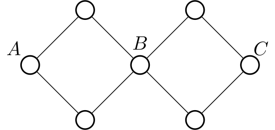
Vertex-biconnectivity is not transitive. The counterexample is shown below: $A,B$ are vertex-biconnected, $B,C$ are vertex-biconnected, but $A,C$ are not vertex-biconnected.

For a maximal edge-biconnected subgraph of an undirected graph, we call this subgraph an edge-biconnected component.

For a maximal vertex-biconnected subgraph of an undirected graph, we call this subgraph a vertex-biconnected component.

DFS Spanning Tree

For a connected undirected graph, we can start DFS from any vertex to obtain a DFS spanning tree of the original graph, with the starting vertex as its root. The edges in this spanning tree are called tree edges, and the edges not in the spanning tree are called non-tree edges.

By the properties of DFS, we can ensure that for the two endpoints of every non-tree edge, one is an ancestor of the other in the spanning tree.

The DFS code is as follows:

Implementation

C++

void DFS(int p) {
  visited[p] = true;
  for (int to : edge[p])
    if (!visited[to]) DFS(to);
}

Python

def DFS(p):
    visited[p] = True
    for to in edge[p]:
        if visited[to] == False:
            DFS(to)

Edge-biconnected Components

Example: Luogu P8436 [Template] Edge-biconnected Components

Given an undirected graph with $n$ vertices and $m$ edges, output the number of its edge-biconnected components and each edge-biconnected component.

Tarjan Algorithm 1

The process of finding biconnected components with Tarjan is similar to that of finding strongly connected components; you can first read the Tarjan algorithm in Strongly Connected Components.

We first find all bridges, and then use DFS to find the edge-biconnected components.

For finding bridges, see the bridge section of Articulation Points and Bridges.

The time complexity is $O(n+m)$ .

Example Code

#include <algorithm>
#include <iostream>
#include <vector>

using namespace std;
constexpr int N = 5e5 + 5, M = 2e6 + 5;
int n, m, ans;
int tot = 1, hd[N];

struct edge {
  int to, nt;
} e[M << 1];

void add(int u, int v) { e[++tot].to = v, e[tot].nt = hd[u], hd[u] = tot; }

void uadd(int u, int v) { add(u, v), add(v, u); }

bool bz[M << 1];
int bcc_cnt, dfn[N], low[N], vis_bcc[N];
vector<vector<int>> bcc;

void tarjan(int x, int in) {
  dfn[x] = low[x] = ++bcc_cnt;
  for (int i = hd[x]; i; i = e[i].nt) {
    int v = e[i].to;
    if (dfn[v] == 0) {
      tarjan(v, i);
      if (dfn[x] < low[v]) bz[i] = bz[i ^ 1] = true;
      low[x] = min(low[x], low[v]);
    } else if (i != (in ^ 1))
      low[x] = min(low[x], dfn[v]);
  }
}

void dfs(int x, int id) {
  vis_bcc[x] = id, bcc[id - 1].push_back(x);
  for (int i = hd[x]; i; i = e[i].nt) {
    int v = e[i].to;
    if (vis_bcc[v] || bz[i]) continue;
    dfs(v, id);
  }
}

int main() {
  cin.tie(nullptr)->sync_with_stdio(false);
  cin >> n >> m;
  int u, v;
  for (int i = 1; i <= m; i++) {
    cin >> u >> v;
    if (u == v) continue;
    uadd(u, v);
  }
  for (int i = 1; i <= n; i++)
    if (dfn[i] == 0) tarjan(i, 0);
  for (int i = 1; i <= n; i++)
    if (vis_bcc[i] == 0) {
      bcc.push_back(vector<int>());
      dfs(i, ++ans);
    }
  cout << ans << '\n';
  for (int i = 0; i < ans; i++) {
    cout << bcc[i].size();
    for (int j = 0; j < bcc[i].size(); j++) cout << ' ' << bcc[i][j];
    cout << '\n';
  }
  return 0;
}

Tarjan Algorithm 2

Let us first summarize an important property: in an undirected graph, an edge in the DFS spanning tree that is not a tree edge is a non-tree edge.

Consider the method for finding strongly connected components. In an undirected graph, as long as a component has no bridges, all its vertices are in the same strongly connected component of the DFS spanning tree.

Conversely, a strongly connected component in the DFS spanning tree is an edge-biconnected component in the original undirected graph.

It can be seen that finding edge-biconnected components is in fact the same process as finding strongly connected components.

The time complexity is $O(n+m)$ .

Example Code

#include <algorithm>
#include <iostream>
#include <stack>
#include <vector>

using namespace std;
constexpr int N = 5e5 + 5, M = 2e6 + 5;
int n, m;

struct edge {
  int to, nt;
} e[M << 2];

int hd[N << 1], tot = 1;

void add(int u, int v) { e[++tot] = edge{v, hd[u]}, hd[u] = tot; }

void uadd(int u, int v) { add(u, v), add(v, u); }

int bcc_cnt, sum;
int dfn[N], low[N];
bool vis[N];
vector<vector<int>> ans;
stack<int> st;

void tarjan(int u, int in) {
  low[u] = dfn[u] = ++bcc_cnt;
  st.push(u), vis[u] = true;
  for (int i = hd[u]; i; i = e[i].nt) {
    int v = e[i].to;
    if (i == (in ^ 1)) continue;
    if (!dfn[v])
      tarjan(v, i), low[u] = min(low[u], low[v]);
    else if (vis[v])
      low[u] = min(low[u], dfn[v]);
  }
  if (dfn[u] == low[u]) {
    vector<int> t;
    t.push_back(u);
    while (st.top() != u)
      t.push_back(st.top()), vis[st.top()] = false, st.pop();
    st.pop(), ans.push_back(t);
  }
}

int main() {
  cin.tie(nullptr)->sync_with_stdio(false);
  cin >> n >> m;
  int u, v;
  for (int i = 1; i <= m; i++) {
    cin >> u >> v;
    if (u != v) uadd(u, v);
  }
  for (int i = 1; i <= n; i++)
    if (!dfn[i]) tarjan(i, 0);
  cout << ans.size() << '\n';
  for (int i = 0; i < ans.size(); i++) {
    cout << ans[i].size() << ' ';
    for (int j = 0; j < ans[i].size(); j++) cout << ans[i][j] << ' ';
    cout << '\n';
  }
  return 0;
}

Difference Algorithm

As with Tarjan Algorithm 1, we first find all bridges and then use differences to find the edge-biconnected components.

First, perform DFS on the original graph.

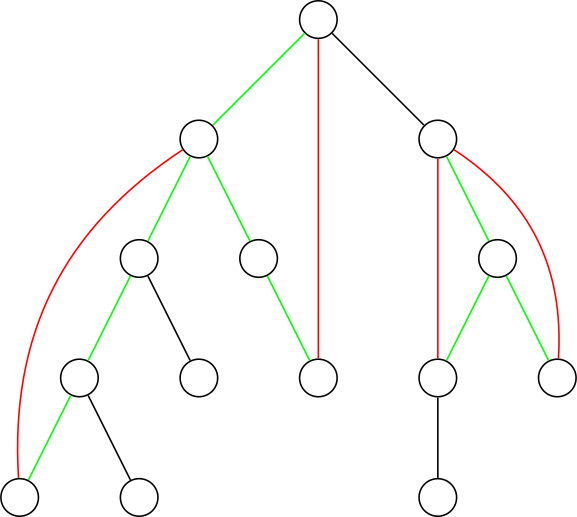
As shown in the figure above, the black and green edges are tree edges, and the red edges are non-tree edges. The two endpoints of every non-tree edge uniquely determine a simple path on the tree consisting of tree edges; we say that this non-tree edge covers every edge on this simple path.

In the graph, every green tree edge is covered by at least one non-tree edge, while no black tree edge is covered by any non-tree edge.

Clearly, non-tree edges and green tree edges are certainly not bridges, while black tree edges are certainly bridges.

Consider a brute-force approach first: for every non-tree edge, set each tree edge it covers to green one by one. Its time complexity is $O(nm)$ .

Consider using differences for optimization. For every non-tree edge, place a -1 mark at its endpoint with smaller depth in the tree and a +1 mark at its endpoint with greater depth in the tree, and then compute, in $O(n)$ , the sum of marks inside the subtree of each vertex.

For a vertex $u$ , the sum of marks inside its subtree equals the number of non-tree edges that cover the tree edge between $u$ and $fa_u$ . If this value is $0$ , then the tree edge between $u$ and $fa_u$ is a bridge.

Then use DFS to find the edge-biconnected components.

The time complexity is $O(n+m)$ .

Example Code

#include <cstring>
#include <iostream>
#include <vector>
using namespace std;
#define min(x, y) (x < y ? x : y)
#define max(x, y) (x > y ? x : y)
constexpr int N = 5e5 + 5, M = 2e6 + 5;
int n, m;

struct edge {
  int to, nt;
} e[M << 1];

int hd[N], tot;

void add(int u, int v) { e[++tot] = {v, hd[u]}, hd[u] = tot; }

void uadd(int u, int v) { add(u, v), add(v, u); }  // Forward-star adjacency list

using ll = long long;
#define P(x, y) ((ll)min(x, y) * N + (ll)max(x, y))
constexpr int hmod = 1e5 + 7;

struct hash {
  vector<ll> v1[hmod];
  vector<short> v2[hmod];

  short &operator[](ll x) {
    int y = x % hmod;
    for (int i = 0; i < v1[y].size(); i++)
      if (v1[y][i] == x) return v2[y][i];
    v1[y].push_back(x), v2[y].push_back(0);
    return v2[y].back();
  }
} re, be;  // Implement the hash table with vectors because this problem has tight time and memory limits

// re tracks whether parallel edges exist; be records whether an edge is a bridge

// #define P(x, y) {min(x, y), max(x, y)}
// using pii = pair<int, int>;
// map<pii, int> re, be; // When constraints are looser, a map can implement the hash table

int dep[N], bz[N], sum[N];  // Record depths, difference values, and subtree difference sums
int vis[N], fa[N];          // Record whether a vertex has been visited and its component ID

void dfs(int x, int pre) {  // Compute each vertex's depth and its point difference value
  if (dep[x] < dep[pre]) bz[x]++, bz[pre]--;  // Returning to an ancestor; update the difference values
  if (dep[x]) return;
  dep[x] = dep[pre] + 1;
  for (int i = hd[x]; i; i = e[i].nt) dfs(e[i].to, x);
}

int dfs2(int x, int pre) {  // Process subtree difference sums
  if (vis[x] == 1) return sum[x];
  vis[x] = 1, sum[x] = bz[x];
  for (int i = hd[x]; i; i = e[i].nt) {
    int v = e[i].to;
    if (dep[v] > dep[x] && !vis[v]) sum[x] += dfs2(v, x);
  }
  if (sum[x] == 0 && re[P(x, pre)] == 1) be[P(x, pre)] = 1;  // Record the bridge
  return sum[x];
}

int cnt;
vector<int> ans[N];

void dfs3(int x) {  // Compute biconnected components
  if (fa[x]) return;
  ans[cnt].push_back(x), fa[x] = cnt;
  for (int i = hd[x]; i; i = e[i].nt) {
    int v = e[i].to;
    if (be[P(x, v)] != 1) dfs3(v);  // Not a bridge; recursively process the subtree
  }
}

int main() {
  cin.tie(nullptr)->sync_with_stdio(false);
  cin >> n >> m;
  int u, v;
  for (int i = 1; i <= m; i++) cin >> u >> v, uadd(u, v), re[P(u, v)]++;
  for (int i = 1; i <= n; i++)
    if (!dep[i]) dfs(i, 0);
  for (int i = 1; i <= n; i++)
    if (!vis[i]) dfs2(i, 0);
  for (int i = 1; i <= n; i++)
    if (!fa[i]) cnt++, dfs3(i);
  cout << cnt << '\n';
  for (int i = 1; i <= cnt; i++) {
    cout << ans[i].size() << ' ';
    for (int j = 0; j < ans[i].size(); j++) cout << ans[i][j] << ' ';
    cout << '\n';
  }
  return 0;
}

#2788. “CEOI2015 Day1” Pipeline

Given an undirected graph with $N$ vertices and $M$ edges, not necessarily connected. Treat each connected component as a subgraph and find the bridges in every subgraph. You have only 16 MB of memory.

Solution

The most important feature of this problem is that you cannot store all the edges.

Consider optimizing edge storage: if one non-tree edge is completely covered by another non-tree edge, then this edge is useless.

A disjoint-set union can be used to maintain this.

Vertex-biconnected Components

Example: Luogu P8435 [Template] Vertex-biconnected Components

Given an undirected graph with $n$ vertices and $m$ edges, output the number of its vertex-biconnected components and each vertex-biconnected component.

Tarjan Algorithm

You need to learn about articulation points first; see the articulation-point section of Articulation Points and Bridges.

First, we give two properties:

Any two vertex-biconnected components have at most one common vertex, and that vertex must be an articulation point.
For a vertex-biconnected component, the vertex with the smallest dfn value in the DFS search tree is necessarily an articulation point or the root of the tree.

We discuss the cases according to the second property:

When this vertex is an articulation point, it must be the root of the vertex-biconnected component, because once its parent is included, it is still an articulation point.
When this vertex is the root of the tree:
1. If it has two or more subtrees, it is an articulation point.
2. If it has only one subtree, it is the root of a vertex-biconnected component.
3. If it has no subtree, regard it as a vertex-biconnected component.

Example Code

#include <iostream>
#include <vector>
using namespace std;
constexpr int N = 5e5 + 5, M = 2e6 + 5;
int n, m;

struct edge {
  int to, nt;
} e[M << 1];

int hd[N], tot = 1;

void add(int u, int v) { e[++tot] = edge{v, hd[u]}, hd[u] = tot; }

void uadd(int u, int v) { add(u, v), add(v, u); }

int ans;
int dfn[N], low[N], bcc_cnt;
int sta[N], top, cnt;
bool cut[N];
vector<int> dcc[N];
int root;

void tarjan(int u) {
  dfn[u] = low[u] = ++bcc_cnt, sta[++top] = u;
  if (u == root && hd[u] == 0) {
    dcc[++cnt].push_back(u);
    return;
  }
  int f = 0;
  for (int i = hd[u]; i; i = e[i].nt) {
    int v = e[i].to;
    if (!dfn[v]) {
      tarjan(v);
      low[u] = min(low[u], low[v]);
      if (low[v] >= dfn[u]) {
        if (++f > 1 || u != root) cut[u] = true;
        cnt++;
        do dcc[cnt].push_back(sta[top--]);
        while (sta[top + 1] != v);
        dcc[cnt].push_back(u);
      }
    } else
      low[u] = min(low[u], dfn[v]);
  }
}

int main() {
  cin.tie(nullptr)->sync_with_stdio(false);
  cin >> n >> m;
  int u, v;
  for (int i = 1; i <= m; i++) {
    cin >> u >> v;
    if (u != v) uadd(u, v);
  }
  for (int i = 1; i <= n; i++)
    if (!dfn[i]) root = i, tarjan(i);
  cout << cnt << '\n';
  for (int i = 1; i <= cnt; i++) {
    cout << dcc[i].size() << ' ';
    for (int j = 0; j < dcc[i].size(); j++) cout << dcc[i][j] << ' ';
    cout << '\n';
  }
  return 0;
}

Difference Algorithm

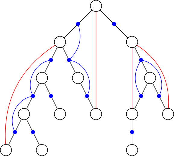
As shown in the figure above, the black edges are tree edges and the red edges are non-tree edges. The two endpoints of every non-tree edge uniquely determine a simple path on the tree consisting of tree edges.

Consider a new graph in which each vertex corresponds to a tree edge in the original graph (represented by a blue vertex in the figure). For every non-tree edge in the original graph, connect the blue vertices corresponding to all edges on the simple tree path associated with that non-tree edge into a connected component; these connections are represented by blue edges in the figure.

Thus, a vertex is not an articulation point if and only if all blue vertices in the new graph corresponding to its incident edges belong to the same connected component.

Two vertices are vertex-biconnected if and only if all blue vertices in the new graph corresponding to the edges on their path in the original tree belong to the same connected component. In other words, every connected component formed by the blue vertices is a vertex-biconnected component.

The connectivity relationship between blue vertices can be maintained using a method similar to the difference method used for finding edge-biconnected components. The time complexity is $O(n+m)$ .

Biconnected Components

Introduction

Definitions

DFS Spanning Tree

Edge-biconnected Components

Tarjan Algorithm 1

Tarjan Algorithm 2

Difference Algorithm

Vertex-biconnected Components

Tarjan Algorithm

Difference Algorithm