This article introduces planar graphs and related concepts.
Planar graphs
If a graph can be drawn on a plane so that no edges intersect except at vertices, then is said to be embeddable in the plane , and is a planar graph. A drawing with no edge intersections is called a planar representation or planar embedding of . This planar embedding of a planar graph is also called a plane graph.
“Plane graph”
The meaning of “plane graph” may differ across Chinese texts. In this article's definitions, a planar graph is a graph-theoretic object that may be embedded in the plane in different ways; a plane graph is a geometric object that, in addition to its graph-theoretic structure, specifies how the graph is drawn. The same planar graph often corresponds to multiple plane graphs. Therefore, when a conclusion in this article depends only on graph-theoretic structure, we use “planar graph”; when it also depends on the graph's planar embedding, we use “plane graph”.
Here are simple examples of plane graphs:
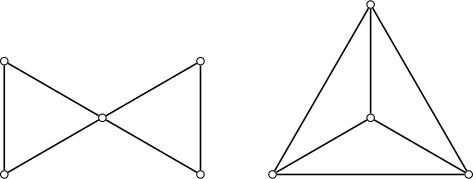
(Left: butterfly graph; right: the complete graph of order , .)
Here are simple examples of non-planar graphs:
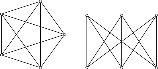
(Left: the complete graph of order , ; right: the complete bipartite graph with vertices in each part, .)
Properties
This section introduces properties of plane graphs.
Faces and their degrees
Let be a plane graph. The edges of divide the plane containing into several regions, each of which is called a face of . An unbounded face is called the unbounded face or external face, while a bounded face is called a finite or internal face. Every plane graph has exactly one external face.
The cycle formed by all edges surrounding a face is called its boundary, and an edge on the boundary is said to be incident to the face. The length of the boundary is called the degree of the face. When calculating a face's degree, every bridge is counted twice. The sum of the degrees of all faces in a plane graph is twice the number of edges times .
In a plane graph, the boundary of a face of degree corresponds to a self-loop, and the boundary of a face of degree usually corresponds to a pair of parallel edges1. In a simple connected plane graph with , every face has degree at least .
Euler's formula
An important property of plane graphs is Euler's formula. It gives the relationship among the number of vertices , the number of edges , and the number of faces .
Euler's formula
For a connected plane graph ,
Proof
Apply induction on the number of faces . The base case is . In this case, the plane graph has exactly one external face and every edge is a bridge. Thus, graph is a tree and necessarily has , which satisfies Euler's formula. Assume Euler's formula holds for plane graphs with faces. For the plane graph with , namely , there must be a non-bridge edge that is incident to two different faces. Delete edge to obtain , which has vertices, edges, and faces. By the induction hypothesis, Euler's formula holds for , namely . Rearranging gives Euler's formula for . Therefore, by induction, Euler's formula holds for all plane graphs.
Corollary
For a plane graph with connected components, namely , we have
Proof
Every connected component of is a plane graph, but these components share the same external face. Therefore, applying Euler's formula to the components and adding the results gives the correct total numbers of vertices and edges, but overcounts the total number of faces by , because the single external face is counted times. Accounting for this correction gives .
This gives a relationship between the numbers of edges and vertices in a plane graph.
Theorem
For a plane graph with connected components, namely , if every face of graph has degree at least , then
Proof
Since every face of has degree at least , the sum of all face degrees is at least , namely . Substituting the corollary of Euler's formula gives
Using , solve for to obtain
Corollary
Let be a simple planar graph with . Then
Proof
When is connected, every face has degree at least . Taking and in the theorem above gives .
When is disconnected, there are two cases:
- If some connected component has at least vertices, then for each connected component with at least vertices, establish separately. Every component with fewer than vertices necessarily has . Adding the inequalities for all connected components gives .
- If every connected component has fewer than vertices, then the whole graph necessarily has . Since implies , we still have .
This proves the proposition.
This corollary shows that simple planar graphs are sparse graphs.
Dual graphs
Every plane graph has a corresponding (geometric) dual graph.
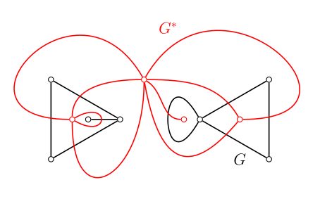
Let be a plane graph. Construct a graph as follows:
- In every face of , denoted , draw a point .
- For every edge of , denoted , if lies on the common boundary of faces and , draw an edge connecting and , namely , so that it intersects exactly once and does not intersect any other edge of or . In particular, when occurs on the boundary of only one face , draw a self-loop incident to that intersects .
The resulting graph is called the dual graph of .
Theorem
Let be the dual graph of a plane graph . Then is a connected plane graph. Moreover, is isomorphic to if and only if is connected.
Proof
The fact that is a plane graph follows from its construction. We also need to prove that graph is connected. For any two vertices in graph , namely , let the line segment connecting and in the plane pass through the faces and edges of graph in the sequence ; these correspond to the vertices and edges in the dual graph. By the construction of , consecutive vertices and edges in the sequence are incident, so this describes a walk in . Hence, graph is connected.
The graph is the dual graph of graph and is necessarily connected. Therefore, is isomorphic to , and a necessary condition is that graph be connected. Next, prove that this condition is sufficient. It is enough to show that when graph is connected, graph satisfies the construction requirements for the dual graph of graph . Because the edges of graph correspond naturally to those of graph , it suffices to show that every face of graph contains exactly one vertex of graph . For any face of graph , namely , let a boundary edge be . Then the corresponding edge in graph , namely , has one endpoint inside face ; hence face contains at least one vertex of graph . Since graph and graph are connected, Euler's formula holds; graph and graph have equal numbers of edges, the number of faces of graph equals the number of vertices of graph , so the number of vertices of graph equals the number of faces of graph . Thus every face of graph contains exactly one vertex of graph . The proposition follows.
The structures of a plane graph and its dual have many correspondences:
- Faces in correspond to vertices in , edges in correspond to edges in , and vertices in correspond to faces in .
- Self-loops in correspond to bridges in , and self-loops in correspond to bridges in .
- Edge cuts in correspond to cycles in , and cycles in correspond to edge cuts in .
Note that the concept of a dual graph applies only to a specific plane graph and cannot be defined for an arbitrary planar graph. In fact, the dual graphs of two isomorphic plane graphs need not be isomorphic. In other words, different planar embeddings of the same graph may have different dual graphs.
Example
The following figure shows two isomorphic plane graphs whose dual graphs are not isomorphic.
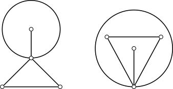
The reason their dual graphs are not isomorphic is that the graph on the right has a face of degree 1, so its dual graph has a vertex of degree 1, while the graph on the left does not.
Transforming a planar graph problem into a problem on its dual graph can sometimes make it easier to solve. A typical example is that the minimum cut problem on a planar graph can be transformed into the shortest path problem on its dual graph. Let be an edge-weighted planar graph, and let be two of its vertices. We need to find the minimum - cut.
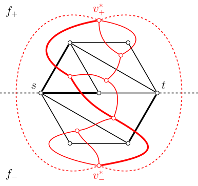
As shown in the figure, choose a suitable planar embedding so that lie on the boundary of the external face of . In addition, draw rays extending from and to divide the external face into two parts and . Construct the dual graph based on this drawing, and assign the corresponding edge weights to the edges of the dual graph. Then a path between the vertices corresponding to faces and in the dual graph corresponds one-to-one with graph 's - edge cut, and the two have the same weight. Thus, finding a shortest path in graph 's dual graph gives the minimum - cut.
A common misconception is to claim, based on the transformation above, that the minimum cut of a plane graph equals the shortest path of its dual graph. In fact, this applies only when has a planar embedding in which are coplanar, although algorithm-contest problems testing this topic often provide a graph together with such an embedding. Here is a theorem that can be used to determine whether such an embedding exists.
Theorem
For a planar graph and two vertices , there exists a planar embedding of in which lie on the same face if and only if is a planar graph.
Proof
If there is a planar embedding of in which lie on the same face, an edge can be added inside that face while preserving planarity.
If is planar, take any planar embedding of it. Then lie on the same face containing the edge . After deleting , still lie on the same face. The proposition follows.
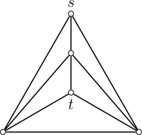
For example, adding edge in the following figure produces the non-planar graph , so such a planar embedding does not exist and the transformation above does not apply.
More results
Of course, plane graphs have many other famous results. This section simply lists some of them without discussion.
Four color theorem
Plane graphs (without self-loops) are -colorable.
Fáry's theorem
Every simple planar graph has a planar embedding in which all edges are line segments.
Theorem (Wood)
A planar graph has at most maximal cliques.
Theorem (Tutte)
Every -vertex-connected planar graph is Hamiltonian.
Recognition
This section discusses how to determine whether a given graph is planar.
Forbidden graphs
The most classical characterization of planar graphs uses forbidden graphs.
First, and are not planar.
Theorem
and are not planar.
Proof
As stated earlier, every simple connected plane graph with must satisfy
Here, is the minimum face degree. For , , so cannot be drawn as a plane graph. For , , so cannot be drawn as a plane graph.
In fact, these are the minimal structures that make a graph non-planar. In other words, as long as a graph does not contain these two graphs as substructures (in a certain sense), it must be planar.
The first planarity characterization theorem is Kuratowski's theorem. It uses the concept of graph homeomorphism: if two graphs and are isomorphic, or become isomorphic after repeatedly inserting or deleting degree- vertices, they are called homeomorphic. The result can be stated as follows:
Kuratowski's theorem
A graph is planar if and only if contains no subgraph homeomorphic to or .
Another related theorem is Wagner's theorem. It characterizes planar graphs using contractions. A contraction repeatedly contracts an edge of a graph into a vertex. The result is:
Wagner's theorem
A graph is planar if and only if has no subgraph that can be contracted to or .
It is relatively obvious that a planar graph does not contain these types of subgraphs, so the key part of both theorems is the sufficiency of the corresponding forbidden-subgraph condition. A subgraph homeomorphic to or can certainly be contracted to them, but the converse need not hold. Thus, Kuratowski's theorem provides a weaker and easier-to-check condition for recognizing planar graphs.
Planarity testing algorithms
Although it may not look easy, the planarity testing problem actually has many linear-time algorithms. However, because their implementations are usually quite complicated, they have almost never appeared in algorithm contests.
The earliest linear-time algorithm was the Hopcroft–Tarjan algorithm2, but its implementation is rather complicated. The de Fraysseix–Ossona de Mendez–Rosenstiehl algorithm (also called the LR planarity algorithm)345 further improves the process of the Hopcroft–Tarjan algorithm and is one of the best planarity testing algorithms available. The Python NetworkX library implements this algorithm.
Another equally excellent algorithm is the Boyer–Myrvold algorithm67. It can determine in linear time whether a given graph is planar. If the graph is planar, the algorithm outputs a planar embedding; otherwise, it outputs a Kuratowski subgraph (that is, a subgraph homeomorphic to or ). The C++ Boost library implements this algorithm.
More related algorithms can be found in the references at the end of the article.
Special planar graphs
This section introduces several special types of planar graphs.
Maximal planar graphs
For a simple planar graph , if adding an edge between any pair of its non-adjacent vertices always produces a non-planar graph, then is called a maximal planar graph. The planar embedding of a maximal planar graph is called a plane graph.
Theorem
A maximal planar graph is necessarily connected. Moreover, when , has no bridges.
Proof
If a planar graph is disconnected, then in any planar embedding of we can choose two vertices belonging to different connected components and connect them inside the external face. The resulting graph is clearly still a plane graph, so graph is not maximal planar. Therefore, if graph is maximal planar, it must be connected.
If a planar graph with vertex count , namely , has a bridge , then after deleting , graph has exactly two connected components, and belong to different components. Suppose the component containing has at least two vertices. Draw the component containing , namely , in the plane, choose any face of graph whose boundary contains , denoted , and draw the other component inside face . Since is simple, the boundary of its external face cannot be a self-loop, so there is at least one other vertex . Connecting to produces a plane graph containing graph as a subgraph. Thus, graph is not maximal planar. Therefore, a maximal planar graph with vertex count has no bridges.
The structure of maximal planar graphs can be described more precisely.
Theorem
For a plane graph with vertex count , namely , it is a maximal planar graph if and only if it is simple and every face has degree .
Proof
The sufficiency is obvious. We only need to establish necessity, namely that every face in a maximal planar graph with vertex count , namely , has degree . Since is a connected simple plane graph and , every face has degree at least . If the proposition were false, there would be a face whose boundary has length at least . Since has no bridges, this boundary must be a cycle. Let it be . If and were not adjacent, then, inside face , connecting and would preserve planarity, contradicting the maximality of ; hence and are adjacent. Similarly, and are adjacent. However, neither edge nor appears in face . Thus both edges must lie outside face . This is impossible, since no matter how they are drawn, the two edges must intersect. Therefore, has no face of degree greater than . The proposition follows.
Corollary
For a graph with vertex count , namely , the number of edges is always and the number of faces is .
Since every face of a maximal planar graph is bounded by three edges, a maximal planar graph is also called a plane triangulation.
Outerplanar graphs
Let be a planar graph. If has a planar embedding such that all vertices of lie on the boundary of one face of , then is called an outerplanar graph. This embedding is also called an outerplane embedding or an outerplane graph. Usually, the face whose boundary passes through all vertices is drawn as the external face.
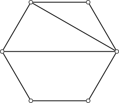
Every outerplanar graph is planar, but the converse does not necessarily hold. Outerplanar graphs also have a forbidden-subgraph characterization.
Theorem
A graph is outerplanar if and only if contains no subgraph homeomorphic to or .
The concept of maximal outerplanar graphs can likewise be considered. For a simple outerplanar graph , if adding an edge between any pair of non-adjacent vertices always produces a graph that is no longer outerplanar, then is called a maximal outerplanar graph. The outerplane embedding of a maximal outerplanar graph is called a maximal outerplane graph. A maximal outerplane graph is exactly a triangulation of a polygon in the plane.
Theorem
For a maximal outerplane graph with vertex count , namely , and suppose every vertex lies on the boundary of the external face. Then has exactly internal faces.
Proof
Apply induction on . The base case is . Then is a triangle and has only internal face, so the proposition holds. Assume it holds for . We now prove it for .
First, must have a degree- vertex. Otherwise, every vertex except neighboring vertices on the external-face boundary would have to be connected to the third vertex. Number the vertices on the external-face boundary consecutively, and for every , define as the smallest index of a vertex connected to vertex and not adjacent to it in the numbering. Consider the possible values of . First, . Since vertex is already connected to , the segment from vertex to cannot cross edge , so necessarily . Similarly, . Since there are only finitely many vertices, this successively shrinking process must terminate after finitely many steps. Let be the largest value satisfying for . Since vertices and are not adjacent, we necessarily have . Repeating the previous argument would still give , contradicting the maximality of . This contradiction shows that must have a degree- vertex.
Let be a vertex of degree . Delete this vertex from graph to obtain an outerplane graph with vertices, . This graph must be maximal outerplane; otherwise, a legal way to add an edge to it would also be legal for graph . By the induction hypothesis, graph has exactly internal faces, and deleting vertex reduces one internal face of graph . Therefore, graph has internal faces. The proposition follows.
Theorem
For an outerplane graph with vertex count , namely , and suppose every vertex lies on the boundary of the external face. Then is maximal outerplane if and only if the boundary of the external face of is a cycle of length and every internal-face boundary is a cycle of length .
Proof
The sufficiency is obvious. Indeed, consider connecting two non-adjacent vertices on the external-face boundary. If the connection is drawn inside the external face, not all vertices can remain on the boundary of one face; otherwise, the segment must intersect the boundary of an internal face.
Now prove necessity. Suppose the boundary of the external face of , , is not a cycle. Then it passes through some vertex more than once; that is, there exist with such that . Without loss of generality, let . The edges incident to can only lie inside the bounded region enclosed by the cycle , while the edges incident to can only lie inside the bounded region enclosed by the cycle . Therefore, and cannot be adjacent. We can add an edge connecting and , denoted , to obtain . This is clearly also a plane graph, and its external-face boundary contains all vertices. This contradicts the maximal outerplanarity of . Thus, the external face of must be a cycle of length . The reason that every internal-face boundary of is a cycle of length is the same as for maximal planar graphs and is omitted.
Corollary
For a maximal outerplanar graph with vertex count , namely , there are:
- .
- has at least vertices of degree at most , and at least vertices of degree .
- The vertex connectivity of is .
Exercises
- Luogu P3209 [HNOI2010] Planar Graph Recognition
- Luogu P3249 [HNOI2016] Mining Area
- Luogu P4001 [ICPC-Beijing 2006] Catching Rabbits
- Luogu P4073 [WC2013] Plane Graph
- Luogu P7295 [USACO21JAN] Paint by Letters P
References and notes
- Planar graph - Wikipedia
- Planarity testing - Wikipedia
- Bondy, John Adrian, and Uppaluri Siva Ramachandra Murty. Graph theory with applications. Vol. 290. London: Macmillan, 1976.
- Diestel, Reinhard. Graph theory. Vol. 173. Springer Nature, 2025.
- Patrignani, Maurizio. "Planarity Testing and Embedding." (2013): 1-42.
Footnotes
-
But this is not the only possibility. Two nested self-loops also form a face of degree two. In addition, a degree-2 face does not necessarily mean that the graph is not simple; for example, in a graph with only one edge, the unique face (the external face) also has degree two. ↩
-
Hopcroft, John, and Robert Tarjan. "Efficient planarity testing." Journal of the ACM (JACM) 21, no. 4 (1974): 549-568. ↩
-
De Fraysseix, Hubert, Patrice Ossona De Mendez, and Pierre Rosenstiehl. "Trémaux trees and planarity." International Journal of Foundations of Computer Science 17, no. 05 (2006): 1017-1029. ↩
-
De Fraysseix, Hubert. "Trémaux trees and planarity." Electronic Notes in Discrete Mathematics 31 (2008): 169-180. ↩
-
Brandes, Ulrik. "The left-right planarity test." Manuscript submitted for publication 3 (2009). ↩
-
Boyer, John M., and Wendy J. Myrvold. "Stop Minding Your p's and q's: A Simplified O (n) Planar Embedding Algorithm." In SODA, vol. 99, pp. 140-146. 1999. ↩
-
Boyer, John M., and Wendy J. Myrvold. "Simplified o (n) planarity by edge addition." Graph Algorithms and Applications 5 (2006): 241. ↩