AIOJ

Before reading the following content, make sure you understand the graph theory concepts.

Related reading: articulation points and bridges.

Introduction

Trees (or forests) are well known for their useful properties and are easy to maintain with many common data structures.

General graphs do not have such good properties. Fortunately, some problems on general graphs can sometimes be transformed into problems on trees.

A round-square tree (Block forest or Round-square tree)¹ is one way to transform a graph into a tree. This article introduces how to construct round-square trees, their properties, and some applications.

For brevity, some conclusions in this article are left unproved; readers may work through or prove them independently.

Definition

The round-square tree was originally a tool for handling cactus graphs (undirected graphs in which each edge belongs to at most one simple cycle), but after uncovering more of its properties, it can sometimes be used on general undirected graphs.

To introduce the round-square tree, we first need to introduce vertex-biconnected components.

One definition of a vertex-biconnected graph is a graph in which every pair of distinct vertices has at least two internally vertex-disjoint paths. “Vertex-disjoint” means both that no vertex repeats within either path (the paths are simple) and that the two paths have empty intersection (of course, both paths necessarily pass through their common start and end vertices, which are excluded from this consideration).

It is difficult to define whether a graph with only one vertex is vertex-biconnected, so we do not consider graphs with $1$ vertex here.

An almost equivalent definition is a graph with no articulation point. This definition fails only when the graph has two vertices connected by a single edge. It has no articulation point, but there are not two disjoint paths because there is only one path. (This can also be understood as counting that one path twice; indeed, the two copies do not intersect at any other vertex.)

Although the original definition is indeed the former one, for convenience we define a vertex-biconnected graph using the latter definition.

A vertex-biconnected component of a graph is a maximal vertex-biconnected subgraph. Unlike strongly connected components and similar structures, a vertex may belong to multiple vertex-biconnected components, while an edge belongs to exactly one vertex-biconnected component (with the former definition, it might belong to none).

In a round-square tree, each original vertex corresponds to a round vertex, and each vertex-biconnected component corresponds to a square vertex. Thus there are $n+c$ vertices in total, where $n$ is the number of vertices in the original graph and $c$ is the number of its vertex-biconnected components.

For each vertex-biconnected component, its corresponding square vertex is connected to every vertex in that component. Each component forms a “daisy graph,” and multiple “daisy graphs” are connected through articulation points in the original graph (because the separating vertices of a vertex-biconnected component are articulation points).

Clearly, every edge in a round-square tree connects one round vertex and one square vertex.

The figure below shows the vertex-biconnected components and round-square tree corresponding to a graph.²

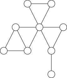
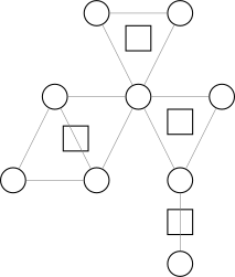
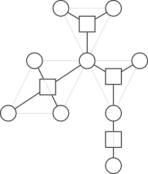
The number of vertices in a round-square tree is less than $2n$ , because the number of articulation points is less than $n$ . Therefore, remember to allocate arrays with twice the necessary size.

In fact, the “round-square tree” is a tree only when the original graph is connected. If the original graph has $k$ connected components, its round-square tree forms a forest consisting of $k$ trees.

If some connected component of the original graph contains only one vertex, the situation must be analyzed case by case; isolated vertices are not considered in the discussion below.

Procedure

How can we construct the round-square tree of a graph? First, if the graph is disconnected, we can split it into connected subgraphs and consider them separately, so we only consider connected graphs.

Because the round-square tree is based on vertex-biconnected components, and vertex-biconnected components are in turn based on articulation points, a method similar to finding articulation points is sufficient.

A common algorithm for finding articulation points is Tarjan’s algorithm. If you know it, the following should be easy to understand; if not, that is fine too.

We skip Tarjan’s articulation-point algorithm and directly introduce the algorithm used for round-square trees (which is actually a variant of Tarjan’s algorithm):

Run DFS on the graph, using two key arrays, dfn and low (as in Tarjan’s algorithm).

dfn[u] stores the DFS number of vertex $u$ , that is, which vertex number it is when $u$ is visited for the first time. low[u] stores the minimum DFS number of a vertex in the DFS-tree subtree of vertex $u$ that some vertex $v$ can reach using at most one back edge or tree edge to its parent. If you have not heard of Tarjan’s algorithm, this may be difficult to understand, so let us look at an example:

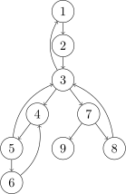
(As you may notice, this graph is equivalent to the graph in the figure above.) Here, tree edges are drawn as straight lines from top to bottom, back edges as curves from bottom to top, and the vertex labels are their DFS numbers.

The low array is as follows:

$i$	$1$	$2$	$3$	$4$	$5$	$6$	$7$	$8$	$9$
$\mathrm{low}[i]$	$1$	$1$	$1$	$3$	$3$	$4$	$3$	$3$	$7$

It is not difficult to understand. Note that the $9$ vertex’s low is $7$ , which differs from some ways of finding articulation points, because for convenience we allow moving upward along the parent edge; the main idea is the same.

It is easy to write a DFS function that computes dfn and low (the dfn array is initially all zero):

Implementation

C++

void Tarjan(int u) {
  low[u] = dfn[u] = ++dfc;                // initialize low with the current node's dfn
  for (int v : G[u]) {                    // iterate over the neighbors of u
    if (!dfn[v]) {                        // if it has not been visited
      Tarjan(v);                          // recurse
      low[u] = std::min(low[u], low[v]);  // take the minimum of low for an unvisited node
    } else
      low[u] = std::min(low[u], dfn[v]);  // take the minimum of dfn for a visited node
  }
}

Python

def Tarjan(u):
    low[u] = dfn[u] = dfc  # initialize low with the current node's dfn
    dfc = dfc + 1
    for v in G[u]:  # iterate over the neighbors of u
        if dfn[v] == False:  # if it has not been visited
            Tarjan(v)  # recurse
            low[u] = min(low[u], low[v])  # take the minimum of low for an unvisited node
        else:
            low[u] = min(low[u], dfn[v])  # take the minimum of dfn for a visited node

Next, we consider the relationship between vertex-biconnected components, the DFS tree, and these two arrays.

We can observe that each vertex-biconnected component is a connected subtree of the DFS tree and contains at least two vertices; in particular, the topmost vertex has only one child below it.

We can also observe that every tree edge belongs to exactly one vertex-biconnected component.

Consider the topmost vertex $u$ of a vertex-biconnected component in the DFS tree. We identify this component at $u$ , because the subtree of $u$ contains all the information about the component.

Since the component contains at least two vertices, consider its next vertex $v$ . There is a tree edge between $u$ and $v$ .

It is not difficult to see that in this case we must have $\mathrm{low}[v]=\mathrm{dfn}[u]$ . More precisely, for a tree edge $u\to v$ , the vertices $u,v$ belong to the same vertex-biconnected component, and $u$ is the shallowest vertex in that component if and only if $\mathrm{low}[v]=\mathrm{dfn}[u]$ .

Thus, during DFS we can determine where vertex-biconnected components exist, but we still cannot determine exactly which vertices each component contains.

This is not difficult to handle: during DFS, maintain a stack containing vertices whose component membership has not yet been determined (possibly for multiple components).

When a vertex-biconnected component is found, all its vertices other than $u$ are concentrated at the top of the stack; repeatedly pop the stack until $v$ is popped.

We can process the popped vertices at the same time by connecting each of them to the newly created square vertex. Finally, connect $u$ to the square vertex as well.

This completes the construction of the round-square tree naturally. We can label square vertices with consecutive integers starting from $n+1$ , which clearly distinguishes round vertices from square vertices.

This part may not have been explained clearly enough. The following code includes detailed comments, output statements to aid understanding, and a sample. Readers are encouraged to copy it and experiment for themselves; code is ultimately the best aid to understanding (do not forget to enable c++11).

Implementation

#include <algorithm>
#include <cstdio>
#include <vector>

constexpr int MN = 100005;

int N, M, cnt;
std::vector<int> G[MN], T[MN * 2];

int dfn[MN], low[MN], dfc;
int stk[MN], tp;

void Tarjan(int u) {
  printf("  Enter : #%d\n", u);
  low[u] = dfn[u] = ++dfc;                // initialize low with the current node's dfn
  stk[++tp] = u;                          // push onto the stack
  for (int v : G[u]) {                    // iterate over the neighbors of u
    if (!dfn[v]) {                        // if it has not been visited
      Tarjan(v);                          // recurse
      low[u] = std::min(low[u], low[v]);  // take the minimum of low for an unvisited node
      if (low[v] == dfn[u]) {  // mark that a biconnected component rooted at u has been found
        ++cnt;                 // increase the number of square vertices
        printf("  Found a New BCC #%d.\n", cnt - N);
        // pop the vertices of the biconnected component other than u and add edges in the round-square tree
        for (int x = 0; x != v; --tp) {
          x = stk[tp];
          T[cnt].push_back(x);
          T[x].push_back(cnt);
          printf("    BCC #%d has vertex #%d\n", cnt - N, x);
        }
        // note that u itself must also be connected (but not popped)
        T[cnt].push_back(u);
        T[u].push_back(cnt);
        printf("    BCC #%d has vertex #%d\n", cnt - N, u);
      }
    } else
      low[u] = std::min(low[u], dfn[v]);  // take the minimum of dfn for a visited node
  }
  printf("  Exit : #%d : low = %d\n", u, low[u]);
  printf("  Stack:\n    ");
  for (int i = 1; i <= tp; ++i) printf("%d, ", stk[i]);
  puts("");
}

int main() {
  scanf("%d%d", &N, &M);
  cnt = N;  // biconnected-component / square-vertex labels start from N
  for (int i = 1; i <= M; ++i) {
    int u, v;
    scanf("%d%d", &u, &v);
    G[u].push_back(v);  // add an undirected edge
    G[v].push_back(u);
  }
  // handle a disconnected graph
  for (int u = 1; u <= N; ++u)
    if (!dfn[u]) Tarjan(u), --tp;
  // note that one element, the root, remains on the stack when Tarjan exits; pop it
  return 0;
}

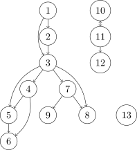
Provide a test case:

The graph corresponding to this example (including multiple edges and an isolated vertex) is:

Examples

We now discuss several example problems that can be solved using round-square trees.

“APIO2018” Ironman

Problem statement

Given a simple undirected graph, count the number of triples $\langle s, c, f \rangle$ (where $s, c, f$ are pairwise distinct) such that there is a simple path starting from $s$ , passing through $c$ , and ending at $f$ .

Solution

When discussing simple paths, we must mention an important property of vertex-biconnected components: for two vertices in a vertex-biconnected component, the union of their simple paths is exactly the component. In other words, for any two distinct vertices $u,v$ in the same vertex-biconnected component, there is a simple path between them that passes through any given other vertex $w$ in that component.

Proof of this property:

Clearly, if a simple path leaves the vertex-biconnected component, it cannot return to it; otherwise this would contradict the definition of a vertex-biconnected component.
Therefore, it suffices to prove that in a vertex-biconnected graph, for any three distinct vertices $u,v,c$ , there is a simple path from $u$ to $v$ passing through $c$ .
First exclude the case of $2$ vertices. It satisfies the property but cannot provide $3$ distinct vertices.
For the remaining cases, construct a network-flow model: connect the source to $c$ with an edge of capacity $2$ , and connect $u$ and $v$ to the sink with edges of capacity $1$ .
Replace each undirected edge $\langle x,y\rangle$ in the original graph with a directed edge from $x$ to $y$ of capacity $1$ and another from $y$ to $x$ of capacity $1$ .
Finally, assign capacity $c$ to every vertex other than the source, sink, and $1$ ; this can be implemented by vertex splitting.
Because the edge from the source to $c$ has capacity $2$ , a maximum flow of $2$ in this network proves that a path through $c$ must exist.
By the max-flow min-cut theorem, the minimum cut is clearly at most $2$ ; it remains to prove that the minimum cut is greater than $1$ .
This is equivalent to proving that deleting any edge of capacity $1$ cannot disconnect the source from the sink.
If the cut removes the edge connecting $u$ or $v$ to the sink, the first definition of a vertex-biconnected graph guarantees a simple path from $c$ to the other vertex not removed.
If the cut removes an edge created by splitting a vertex, this is equivalent to deleting a vertex; by the second definition of a vertex-biconnected graph, the remaining graph is still connected.
If the cut removes an edge created from an original edge, this is equivalent to deleting an edge, which is weaker than deleting a vertex, so a path clearly remains.
Thus the minimum cut is greater than $1$ , so the maximum flow equals $2$ . This proves the claim.

What does this conclusion tell us? It tells us that for the path between two round vertices in the round-square tree, the set of round vertices adjacent to the square vertices (vertex-biconnected components) on the path is exactly the set of vertices on simple paths between the two vertices in the original graph.

Returning to the problem, fix $s$ and $f$ . The number of valid $c$ is clearly equal to the number of valid $c$ , namely the number of vertices in the union of simple paths between the endpoints $s,f$ , minus $2$ (removing $s,f$ themselves).

Therefore, after constructing the round-square tree of the original graph, the number of vertices on simple paths between two vertices is related to the number of square vertices (components) and round vertices on their path in the round-square tree.

Next is a common technique for round-square trees: assign suitable weights to vertices when doing path aggregation. In this problem, each square vertex has weight equal to the size of its corresponding vertex-biconnected component, and each round vertex has weight $-1$ .

With these weights, the sum of vertex weights along a round-square-tree path between two round vertices is exactly the size of the union of simple paths in the original graph minus $2$ .

The problem becomes computing $\sum$ over round-square-tree paths between pairs of round vertices.

Equivalently, compute the contribution of each vertex to the answer: its weight multiplied by the number of paths passing through it. This can be found with a simple tree DP.

Finally, do not forget to handle disconnected graphs. The corresponding code follows:

Reference Code

#include <algorithm>
#include <iostream>
#include <vector>

constexpr int MN = 100005;

int N, M, cnt;
std::vector<int> G[MN], T[MN * 2];
long long Ans;

int dfn[MN], low[MN], dfc, num;
int stk[MN], tp;

int wgh[MN * 2];

void Tarjan(int u) {  // find biconnected components
  low[u] = dfn[u] = ++dfc;
  stk[++tp] = u;
  ++num;
  for (int v : G[u]) {
    if (!dfn[v]) {
      Tarjan(v);
      low[u] = std::min(low[u], low[v]);
      if (low[v] == dfn[u]) {
        wgh[++cnt] = 0;
        for (int x = 0; x != v; --tp) {
          x = stk[tp];
          T[cnt].push_back(x);
          T[x].push_back(cnt);
          ++wgh[cnt];
        }
        T[cnt].push_back(u);
        T[u].push_back(cnt);
        ++wgh[cnt];
      }
    } else
      low[u] = std::min(low[u], dfn[v]);
  }
}

int vis[MN * 2], siz[MN * 2];

void DFS(int u, int fz) {  // DFS to compute the value
  vis[u] = 1;
  siz[u] = (u <= N);
  for (int v : T[u])
    if (v != fz) {
      DFS(v, u);
      Ans += 2ll * wgh[u] * siz[u] * siz[v];
      siz[u] += siz[v];
    }
  Ans += 2ll * wgh[u] * siz[u] * (num - siz[u]);
}

using std::cin;
using std::cout;

int main() {
  cin.tie(nullptr)->sync_with_stdio(false);
  cin >> N >> M;
  for (int u = 1; u <= N; ++u) wgh[u] = -1;
  cnt = N;
  for (int i = 1; i <= M; ++i) {
    int u, v;
    cin >> u >> v;
    G[u].push_back(v);
    G[v].push_back(u);
  }
  for (int u = 1; u <= N; ++u)
    if (!dfn[u]) {
      num = 0;
      Tarjan(u), --tp;
      DFS(u, 0);
    }
  cout << Ans << '\n';
  return 0;
}

The answer for the test case above in this problem is $212$ .

Codeforces #487 E. Tourists

Problem statement

Given a simple connected undirected graph, support two operations:

Modify the weight of a vertex.
Query the minimum vertex weight over all simple paths between two vertices.

Solution

Similarly, construct the round-square tree of the original graph, and set each square vertex’s weight to the minimum weight of its adjacent round vertices. The problem becomes finding the minimum on a path.

A path minimum can be maintained with heavy-light decomposition and a segment tree, but what about updates?

Updating a round vertex’s weight requires updating all adjacent square vertices, which can easily lead to $O(n)$ updates in the worst case.

We use the fact that the round-square tree is a tree: set each square vertex’s weight to the minimum weight among its child round vertices. Then an update only needs to update the parent square vertex.

To maintain a square vertex, simply create a multiset for each square vertex to maintain its set of weights.

Note that when querying, if the LCA is a square vertex, we must also query the weight of the LCA’s parent round vertex.

Note: the round-square tree must be allocated twice as large as the original graph, or the array will overflow.

Reference Code

#include <algorithm>
#include <iostream>
#include <set>
#include <vector>

constexpr int MN = 100005;
constexpr int MS = 524288;
constexpr int Inf = 0x7fffffff;

int N, M, Q, cnt;
int w[MN * 2];
std::vector<int> G[MN], T[MN * 2];
std::multiset<int> S[MN * 2];

int dfn[MN * 2], low[MN], dfc;
int stk[MN], tp;

void Tarjan(int u) {
  low[u] = dfn[u] = ++dfc;
  stk[++tp] = u;
  for (int v : G[u]) {
    if (!dfn[v]) {
      Tarjan(v);
      low[u] = std::min(low[u], low[v]);
      if (low[v] == dfn[u]) {
        ++cnt;
        for (int x = 0; x != v; --tp) {
          x = stk[tp];
          T[cnt].push_back(x);
          T[x].push_back(cnt);
        }
        T[cnt].push_back(u);
        T[u].push_back(cnt);
      }
    } else
      low[u] = std::min(low[u], dfn[v]);
  }
}

int idf[MN * 2], faz[MN * 2], siz[MN * 2], dep[MN * 2], son[MN * 2],
    top[MN * 2];

void DFS0(int u, int fz) {
  faz[u] = fz, dep[u] = dep[fz] + 1, siz[u] = 1;
  for (int v : T[u])
    if (v != fz) {
      DFS0(v, u);
      siz[u] += siz[v];
      if (siz[son[u]] < siz[v]) son[u] = v;
    }
}

void DFS1(int u, int fz, int tp) {
  dfn[u] = ++dfc, idf[dfc] = u, top[u] = tp;
  if (son[u]) DFS1(son[u], u, tp);
  for (int v : T[u])
    if (v != fz && v != son[u]) DFS1(v, u, v);
}

#define li (i << 1)
#define ri (i << 1 | 1)
#define mid ((l + r) >> 1)
#define ls li, l, mid
#define rs ri, mid + 1, r

int dat[MS];

void Build(int i, int l, int r) {  // build the tree
  if (l == r) {
    dat[i] = w[idf[l]];
    return;
  }
  Build(ls), Build(rs);
  dat[i] = std::min(dat[li], dat[ri]);
}

void Mdf(int i, int l, int r, int p, int x) {  // get the minimum
  if (l == r) {
    dat[i] = x;
    return;
  }
  if (p <= mid)
    Mdf(ls, p, x);
  else
    Mdf(rs, p, x);
  dat[i] = std::min(dat[li], dat[ri]);
}

int Qur(int i, int l, int r, int a, int b) {  // query
  if (r < a || b < l) return Inf;
  if (a <= l && r <= b) return dat[i];
  return std::min(Qur(ls, a, b), Qur(rs, a, b));
}

using std::cin;
using std::cout;

int main() {
  cin.tie(nullptr)->sync_with_stdio(false);
  cin >> N >> M >> Q;
  for (int i = 1; i <= N; ++i) cin >> w[i];
  cnt = N;
  for (int i = 1; i <= M; ++i) {
    int u, v;
    cin >> u >> v;
    G[u].push_back(v);
    G[v].push_back(u);
  }
  Tarjan(1), DFS0(1, 0), dfc = 0, DFS1(1, 0, 1);
  for (int i = 1; i <= N; ++i)
    if (faz[i]) S[faz[i]].insert(w[i]);
  for (int i = N + 1; i <= cnt; ++i) w[i] = *S[i].begin();
  Build(1, 1, cnt);
  for (int q = 1; q <= Q; ++q) {
    char opt[3];
    int x, y;
    cin >> opt >> x >> y;
    if (*opt == 'C') {
      Mdf(1, 1, cnt, dfn[x], y);
      if (faz[x]) {
        int u = faz[x];
        S[u].erase(S[u].lower_bound(w[x]));
        S[u].insert(y);
        if (w[u] != *S[u].begin()) {
          w[u] = *S[u].begin();
          Mdf(1, 1, cnt, dfn[u], w[u]);
        }
      }
      w[x] = y;
    } else {
      int Ans = Inf;
      while (top[x] != top[y]) {
        if (dep[top[x]] < dep[top[y]]) std::swap(x, y);
        Ans = std::min(Ans, Qur(1, 1, cnt, dfn[top[x]], dfn[x]));
        x = faz[top[x]];
      }
      if (dfn[x] > dfn[y]) std::swap(x, y);
      Ans = std::min(Ans, Qur(1, 1, cnt, dfn[x], dfn[y]));
      if (x > N) Ans = std::min(Ans, w[faz[x]]);
      cout << Ans << '\n';
    }
  }
  return 0;
}

“SDOI2018” Strategic Game

Problem statement

Given a simple connected undirected graph. There are $q$ queries:

Each query gives a vertex set $S$ ( $2 \le |S| \le n$ ), and asks how many vertices $u$ satisfy $u \notin S$ and, after deleting $u$ , the vertices in $S$ are not all in one connected component.

Each test case contains multiple data sets.

Solution

First construct the round-square tree. The question then becomes asking for the number of round vertices in the connected subgraph corresponding to $S$ on the round-square tree, minus $|S|$ .

How can we calculate the number of round vertices in the connected subgraph? One method is:

Put the weight of each round vertex on the edge between it and its parent square vertex. The problem becomes finding the sum of edge weights; one solution can be found in “SDOI2015” Treasure Hunt. Specifically, sort the vertices in $S$ by DFS order, then compute the sum of distances between consecutive vertices in sorted order (also including the distance between the first and last vertices). The answer is half this sum, because every edge is traversed twice.

Finally, if the shallowest vertex in the subgraph is a round vertex, add $1$ to the answer because it was not counted.

Since there are multiple data sets, remember to initialize the arrays.

Reference Code

#include <algorithm>
#include <iostream>
#include <vector>

constexpr int MN = 100005;

int N, M, Q, cnt;
std::vector<int> G[MN], T[MN * 2];

int dfn[MN * 2], low[MN], dfc;
int stk[MN], tp;

void Tarjan(int u) {  // find biconnected components to prepare the tree
  low[u] = dfn[u] = ++dfc;
  stk[++tp] = u;
  for (int v : G[u]) {
    if (!dfn[v]) {
      Tarjan(v);
      low[u] = std::min(low[u], low[v]);
      if (low[v] == dfn[u]) {
        ++cnt;
        for (int x = 0; x != v; --tp) {
          x = stk[tp];
          T[cnt].push_back(x);
          T[x].push_back(cnt);
        }
        T[cnt].push_back(u);
        T[u].push_back(cnt);
      }
    } else
      low[u] = std::min(low[u], dfn[v]);
  }
}

int dep[MN * 2], faz[MN * 2][18], dis[MN * 2];

void DFS(int u, int fz) {
  dfn[u] = ++dfc;
  dep[u] = dep[faz[u][0] = fz] + 1;
  dis[u] = dis[fz] + (u <= N);
  for (int j = 0; j < 17; ++j) faz[u][j + 1] = faz[faz[u][j]][j];
  for (int v : T[u])
    if (v != fz) DFS(v, u);
}

int LCA(int x, int y) {  // lowest common ancestor
  if (dep[x] < dep[y]) std::swap(x, y);
  for (int j = 0, d = dep[x] - dep[y]; d; ++j, d >>= 1)
    if (d & 1) x = faz[x][j];
  if (x == y) return x;
  for (int j = 17; ~j; --j)
    if (faz[x][j] != faz[y][j]) x = faz[x][j], y = faz[y][j];
  return faz[x][0];
}

using std::cin;
using std::cout;

int main() {
  cin.tie(nullptr)->sync_with_stdio(false);
  int Ti;
  cin >> Ti;
  while (Ti--) {
    cin >> N >> M;
    for (int i = 1; i <= N; ++i) {
      G[i].clear();
      dfn[i] = low[i] = 0;
    }
    for (int i = 1; i <= N * 2; ++i) T[i].clear();
    for (int i = 1, x, y; i <= M; ++i) {
      cin >> x >> y;
      G[x].push_back(y);
      G[y].push_back(x);
    }
    cnt = N;
    dfc = 0, Tarjan(1), --tp;
    dfc = 0, DFS(1, 0);
    cin >> Q;
    while (Q--) {
      static int S, A[MN];
      cin >> S;
      int Ans = -2 * S;
      for (int i = 1; i <= S; ++i) cin >> A[i];
      std::sort(A + 1, A + S + 1, [](int i, int j) { return dfn[i] < dfn[j]; });
      for (int i = 1; i <= S; ++i) {
        int u = A[i], v = A[i % S + 1];
        Ans += dis[u] + dis[v] - 2 * dis[LCA(u, v)];
      }
      if (LCA(A[1], A[S]) <= N) Ans += 2;
      cout << Ans / 2 << '\n';
    }
  }
  return 0;
}

Exercises

External Links

immortalCO, A Round-Square Tree—the Tool for Handling Cacti, Universal OJ.

References and Notes

Footnotes

This structure was defined and named in 2017 by Chen Junkun in his IOI 2017 Chinese National Team training-camp paper, “The Proposition Report of ‘Magical Subgraphs’ and Its Extensions.” ↩
Chen Junkun, “The Ordinary Round-Square Tree and the Magical (~~Dynamic~~) Dynamic Programming,” NOI 2018 Winter Camp, p. 4. ↩