Prüfer Sequence

This article introduces the Prüfer sequence (Prüfer code), a method of representing a labeled tree by a unique integer sequence.

The Prüfer sequence can be used to prove Cayley's formula. We will also explain how to count the ways to add edges to a graph so that it becomes connected.

Note: We do not consider trees with $1$ vertex.

Prüfer Sequence

Introduction

A Prüfer sequence represents a tree with $n$ labeled vertices by integers from $[1,n]$, specifically $n-2$ integers. It can also be understood as a bijection between the spanning trees of a complete graph and sequences, which is useful in common combinatorial counting problems.

Heinz Prüfer invented this sequence in 1918 to prove Cayley's formula.

Constructing a Prüfer Sequence from a Tree

The Prüfer sequence is constructed as follows: each time, choose and delete the leaf with the smallest label, and record the vertex to which it was connected in the sequence. After repeating this $n-2$ times, only two vertices remain and the algorithm ends.

Clearly, using a heap gives complexity $O(n\log n)$.

// Code excerpted from the original; vertices are numbered from 0
vector<vector<int>> adj;

vector<int> pruefer_code() {
  int n = adj.size();
  set<int> leafs;
  vector<int> degree(n);
  vector<bool> killed(n);
  for (int i = 0; i < n; i++) {
    degree[i] = adj[i].size();
    if (degree[i] == 1) leafs.insert(i);
  }

  vector<int> code(n - 2);
  for (int i = 0; i < n - 2; i++) {
    int leaf = *leafs.begin();
    leafs.erase(leafs.begin());
    killed[leaf] = true;
    int v;
    for (int u : adj[leaf])
      if (!killed[u]) v = u;
    code[i] = v;
    if (--degree[v] == 1) leafs.insert(v);
  }
  return code;
}

# Vertices are numbered from 0
adj = [[]]


def pruefer_code():
    n = len(adj)
    leafs = set()
    degree = [0] * n
    killed = [False] * n
    for i in range(1, n):
        degree[i] = len(adj[i])
        if degree[i] == 1:
            leafs.intersection(i)
    code = [0] * (n - 2)
    for i in range(1, n - 2):
        leaf = leafs[0]
        leafs.pop()
        killed[leaf] = True
        for u in adj[leaf]:
            if killed[u] == False:
                v = u
        code[i] = v
        if degree[v] == 1:
            degree[v] = degree[v] - 1
            leafs.intersection(v)
    return code

For example, this is the construction process for the Prüfer sequence of a tree with 7 vertices:

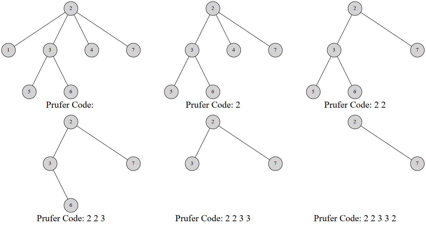
The resulting sequence is $2,2,3,3,2$.

There is also a linear-time construction algorithm.

Linear-Time Construction of a Prüfer Sequence

The essence of the linear construction is to maintain a pointer to the vertex we are about to delete. First observe that the number of leaves is non-increasing: deleting a leaf either leaves the total number of leaves unchanged or decreases it by 1.

We therefore consider the following process. Maintain a pointer $p$. Initially, $p$ points to the leaf with the smallest label. At the same time, maintain the degree of every vertex so that we can determine whether deleting a vertex creates a new leaf. The operations are:

1. Delete the vertex pointed to by $p$, and check whether a new leaf is created.
2. If a new leaf is created, suppose its label is $x$ and compare $p,x$. If $x>p$, do nothing else; otherwise, immediately delete $x$, check whether deleting $x$ creates another new leaf, and repeat step $2$ until no new vertex is created or the new vertex has label $>p$.
3. Increment the pointer $p$ until an undeleted leaf is encountered;

Correctness

Repeating the above operations $n-2$ times completes the construction of the sequence. We now consider the correctness of the algorithm.

$p$ is the leaf with the smallest current label. If deleting $p$ creates no leaf, we can only search for the next leaf; if it creates a leaf $x$:

• If $x>p$, scanning forward from $p$ will reach it anyway, so do nothing;
• If $x> adj; vector<int> parent;

void dfs(int v) { for (int u : adj[v]) { if (u != parent[v]) parent[u] = v, dfs(u); } }

vector<int> pruefer_code() { int n = adj.size(); parent.resize(n), parent[n - 1] = -1; dfs(n - 1);

int ptr = -1; vector<int> degree(n); for (int i = 0; i < n; i++) { degree[i] = adj[i].size(); if (degree[i] == 1 && ptr == -1) ptr = i; }

vector<int> code(n - 2); int leaf = ptr; for (int i = 0; i < n - 2; i++) { int next = parent[leaf]; code[i] = next; if (--degree[next] == 1 && next < ptr) { leaf = next; } else { ptr++; while (degree[ptr] != 1) ptr++; leaf = ptr; } } return code; }

**Python**

```python
# Likewise, starting from 0
adj = [[]]
parent = [0] * n

def dfs(v):
    for u in adj[v]:
        if u != parent[v]:
            parent[u] = v
            dfs(u)

def pruefer_code():
    n = len(adj)
    parent[n - 1] = -1
    dfs(n - 1)

    ptr = -1
    degree = [0] * n
    for i in range(0, n):
        degree[i] = len(adj[i])
        if degree[i] == 1 and ptr == -1:
            ptr = i

    code = [0] * (n - 2)
    leaf = ptr
    for i in range(0, n - 2):
        next = parent[leaf]
        code[i] = next
        if degree[next] == 1 and next < ptr:
            degree[next] = degree[next] - 1
            leaf = next
        else:
            ptr = ptr + 1
            while degree[ptr] != 1:
                ptr = ptr + 1
            leaf = ptr
    return code

Properties of the Prüfer Sequence

1. After constructing the Prüfer sequence, two vertices remain in the original tree, one of which is necessarily the vertex with the largest label, $n$.
2. Each vertex appears in the sequence a number of times equal to its degree minus $1$. (Vertices that do not appear are leaves.)

Reconstructing a Tree from a Prüfer Sequence

The reconstruction method is similar. From the properties of the Prüfer sequence, we can obtain the degree of every vertex in the original tree. We can then find the leaf with the smallest label; this leaf must be connected to the vertex corresponding to the first number in the Prüfer sequence. We then decrease the degrees of these two vertices by one.

By this point you may already know how to proceed. Each time, choose the smallest-labeled vertex of degree $1$, connect it to the vertex currently selected from the Prüfer sequence, and decrease the degrees of both vertices. At the end, two vertices of degree $1$ remain, one of which is vertex $n$; connect them. Maintaining this process with a heap, and adding a vertex to the heap whenever its degree decreases to $1$, gives complexity $O(n\log n)$.

// Code excerpted from the original
vector<pair<int, int>> pruefer_decode(vector<int> const& code) {
  int n = code.size() + 2;
  vector<int> degree(n, 1);
  for (int i : code) degree[i]++;

  set<int> leaves;
  for (int i = 0; i < n; i++)
    if (degree[i] == 1) leaves.insert(i);

  vector<pair<int, int>> edges;
  for (int v : code) {
    int leaf = *leaves.begin();
    leaves.erase(leaves.begin());

    edges.emplace_back(leaf, v);
    if (--degree[v] == 1) leaves.insert(v);
  }
  edges.emplace_back(*leaves.begin(), n - 1);
  return edges;
}

Linear-Time Tree Reconstruction

Use the same method as for the linear construction of a Prüfer sequence. When deleting degree, a new leaf may be created; compare this leaf with the pointer $p$ and process it first if its label is smaller.

Implementation

// Code excerpted from the original
vector<pair<int, int>> pruefer_decode(vector<int> const& code) {
  int n = code.size() + 2;
  vector<int> degree(n, 1);
  for (int i : code) degree[i]++;

  int ptr = 0;
  while (degree[ptr] != 1) ptr++;
  int leaf = ptr;

  vector<pair<int, int>> edges;
  for (int v : code) {
    edges.emplace_back(leaf, v);
    if (--degree[v] == 1 && v < ptr) {
      leaf = v;
    } else {
      ptr++;
      while (degree[ptr] != 1) ptr++;
      leaf = ptr;
    }
  }
  edges.emplace_back(leaf, n - 1);
  return edges;
}

These processes make it clear that the Prüfer sequence establishes a bijection between labeled unrooted trees and sequences.

Cayley Formula (Cayley's formula)

The complete graph $K_n$ has $n^{n-2}$ spanning trees.

How can we prove this? There are many methods, but a Prüfer-sequence proof is very simple. Every integer sequence of length $n-2$ with value range $[1,n]$ corresponds bijectively to a spanning tree through the Prüfer sequence, so the number of possibilities is $n^{n-2}$.

Number of Ways to Make a Graph Connected

The Prüfer sequence may be more powerful than you expect. It yields formulas more general than Cayley's formula. Consider the following problem:

An undirected labeled graph with $n$ vertices, $m$ edges, and $k$ connected components is given. We want to add $k-1$ edges so that the entire graph becomes connected. Count the number of ways.

Proof

Let $s_i$ denote the number of vertices in the $i$-th connected component. We consider constructing a Prüfer sequence on the $k$ connected components. Since there are many ways to connect two components, this is not an ordinary Prüfer sequence. Let $d_i$ be the degree of the $i$-th connected component. Since the sum of the degrees is twice the number of edges, $\sum_{i=1}^kd_i=2k-2$. For a fixed sequence $d$, the number of ways to construct the Prüfer sequence is

For the $i$-th connected component, there are ${s_i}^{d_i}$ ways to choose its connections. Therefore, for a fixed sequence $d$, the number of ways to make the graph connected is

We now enumerate the sequences $d$, giving

This is not a particularly pleasant expression. But do not panic! We have the multinomial theorem:

Now make the substitution $e_i=d_i-1$ in the original expression. Clearly, $\sum_{i=1}^ke_i=k-2$, so it becomes

Simplifying gives

That is

which is the answer.

Exercises

• Luogu P6086 (Template) Prüfer Sequence (template problem)
• Luogu P11039 (MX-X3-T6) "RiOI-4" TECHNOPOLIS 2085
• UVa #10843 - Anne's game
• Timus #1069 - Prufer Code
• Codeforces - Clues
• Topcoder - TheCitiesAndRoadsDivTwo