AIOJ

Definitions

Before reading the following material, be sure to read the sections on graph-theory concepts and tree basics, and understand the following definitions:

Spanning subgraph
Spanning tree

We define the minimum spanning tree (MST) of a connected undirected graph as a spanning tree with the minimum sum of edge weights.

Note that only a connected graph has a spanning tree; a disconnected graph has only a spanning forest.

Kruskal's algorithm

Kruskal's algorithm is a common and easy-to-implement minimum-spanning-tree algorithm, invented by Kruskal. Its basic idea is to add edges in increasing order of weight; it is a greedy algorithm.

Prerequisites

Disjoint-set union, greedy algorithms, and graph storage.

Implementation

Illustration:

Pseudocode:

\begin{array}{ll} 1 & \textbf{Input. } \text{The edges of the graph } e , \text{ where each element in } e \text{ is } (u, v, w) \\ & \text{ denoting that there is an edge between } u \text{ and } v \text{ weighted } w . \\ 2 & \textbf{Output. } \text{The edges of the MST of the input graph}.\\ 3 & \textbf{Method. } \\ 4 & result \gets \varnothing \\ 5 & \text{sort } e \text{ into nondecreasing order by weight } w \\ 6 & \textbf{for} \text{ each } (u, v, w) \text{ in the sorted } e \\ 7 & \qquad \textbf{if } u \text{ and } v \text{ are not connected in the union-find set } \\ 8 & \qquad\qquad \text{connect } u \text{ and } v \text{ in the union-find set} \\ 9 & \qquad\qquad result \gets result\;\bigcup\ \{(u, v, w)\} \\ 10 & \textbf{return } result \end{array}

The algorithm is simple, but it needs a suitable data structure. Specifically, maintain a forest, test whether two vertices are in the same tree, and connect two trees.

Abstractly, maintain a collection of sets, test whether two elements belong to the same set, and merge two sets.

Connectivity queries and edge insertions can be maintained with a disjoint-set union structure.

Using a sorting algorithm with complexity $O(m\log m)$ and a disjoint-set union with complexity $O(m\alpha(m, n))$ or $O(m\log n)$ gives a Kruskal algorithm with time complexity $O(m\log m)$ .

Proof

The idea is simple. To construct a minimum spanning tree, start with the edge of minimum weight and add edges in increasing order of weight. If adding an edge creates a cycle, discard it. Continue until $n-1$ edges have been added, forming a tree.

Proof: by induction, show that at every point the edge set selected by algorithm K is contained in some MST.

Base case: this is clearly true when the algorithm starts, because a minimum spanning tree exists.

Inductive step: suppose the claim holds at some point, with current edge set $F$ . Let $T$ be this MST, and consider the next edge $e$ to be added.

If $e$ belongs to $T$ , the claim holds.

Otherwise, $T+e$ contains a cycle. Consider another edge on this cycle that does not belong to $F$ , namely $f$ (at least one such edge exists).

First, the weight of $f$ cannot be smaller than that of $e$ ; otherwise $f$ would have been selected before $e$ .

Next, the weight of $f$ cannot be greater than that of $e$ ; otherwise $T+e-f$ would be a spanning tree better than $T$ .

Therefore $T+e-f$ contains $F$ and is also a minimum spanning tree, completing the induction.

Example

Luogu P1195: Pocket Sky

There are $n$ clouds. Connect them into $k$ groups; connecting clouds $X_i$ and $Y_i$ costs $L_i$ . Find the minimum total cost.

Example implementation

C++

#include <algorithm>
#include <iostream>
using namespace std;

int fa[1010];  // Parent pointers
int n, m, k;

struct edge {
  int u, v, w;
};

int l;
edge g[10010];

void add(int u, int v, int w) {
  l++;
  g[l].u = u;
  g[l].v = v;
  g[l].w = w;
}

// Standard disjoint-set union
int findroot(int x) { return fa[x] == x ? x : fa[x] = findroot(fa[x]); }

void Merge(int x, int y) {
  x = findroot(x);
  y = findroot(y);
  fa[x] = y;
}

bool cmp(edge A, edge B) { return A.w < B.w; }

// Kruskal's algorithm
void kruskal() {
  int tot = 0;  // Number of selected edges
  int ans = 0;  // Total cost
  for (int i = 1; i <= m; i++) {
    int xr = findroot(g[i].u), yr = findroot(g[i].v);
    if (xr != yr) {        // The roots differ
      Merge(xr, yr);       // Merge
      tot++;               // Increase the edge count
      ans += g[i].w;       // Increase the cost
      if (tot == n - k) {  // Check whether the selected edge count yields k components
        cout << ans << '\n';
        return;
      }
    }
  }
  cout << "No Answer\n";  // Cannot connect
}

int main() {
  cin >> n >> m >> k;
  if (n == k) {  // Handle the boundary case
    cout << "0\n";
    return 0;
  }
  for (int i = 1; i <= n; i++) {  // Initialize
    fa[i] = i;
  }
  for (int i = 1; i <= m; i++) {
    int u, v, w;
    cin >> u >> v >> w;
    add(u, v, w);  // Add the edge
  }
  sort(g + 1, g + m + 1, cmp);  // Sort by edge weight first
  kruskal();
  return 0;
}

Python

class Edge:
    def __init__(self, u, v, w):
        self.u = u
        self.v = v
        self.w = w


fa = [0] * 1010  # Parent pointers
g = []


def add(u, v, w):
    g.append(Edge(u, v, w))


# Standard disjoint-set union
def findroot(x):
    if fa[x] == x:
        return x
    fa[x] = findroot(fa[x])
    return fa[x]


def Merge(x, y):
    x = findroot(x)
    y = findroot(y)
    fa[x] = y


# Kruskal's algorithm
def kruskal():
    tot = 0  # Number of selected edges
    ans = 0  # Total cost
    for e in g:
        x = findroot(e.u)
        y = findroot(e.v)
        if x != y:  # The roots differ
            fa[x] = y  # Merge
            tot += 1  # Increase the edge count
            ans += e.w  # Increase the cost
            if tot == n - k:  # Check whether the selected edge count yields k components
                print(ans)
                return
    print("No Answer")  # Cannot connect


if __name__ == "__main__":
    n, m, k = map(int, input().split())
    if n == k:  # Handle the boundary case
        print("0")
        exit()
    for i in range(1, n + 1):  # Initialize
        fa[i] = i
    for i in range(1, m + 1):
        u, v, w = map(int, input().split())
        add(u, v, w)  # Add the edge
    g.sort(key=lambda edge: edge.w)  # Sort by edge weight first
    kruskal()

Java

import java.util.Arrays;
import java.util.Scanner;

class Edge {
    int u;
    int v;
    int w;

    Edge(int u, int v, int w) {
        this.u = u;
        this.v = v;
        this.w = w;
    }
}

public class Main {
    static int[] parent = new int[1010];  // Parent pointers
    static int m, n, k;  // n is the number of vertices, m the number of edges, and k the required number of components

    static Edge[] edges = new Edge[10010];
    static int l;

    static void addEdge(int u, int v, int w) {
        edges[++l] = new Edge(u, v, w);
    }

    // Standard disjoint-set union
    static int findroot(int x) {
        if (parent[x] != x) {
            parent[x] = findroot(parent[x]);
        }
        return parent[x];
    }

    static void Merge(int x, int y) {
        x = findroot(x);
        y = findroot(y);
        parent[x] = y;
    }

    static boolean cmp(Edge A, Edge B) {
        return A.w < B.w;
    }

    // Kruskal's algorithm
    static void kruskal() {
        int tot = 0;  // Number of selected edges
        int ans = 0;  // Total cost

        for (int i = 1; i <= m; i++) {
            int xr = findroot(edges[i].u);
            int yr = findroot(edges[i].v);
            if (xr != yr) {   // The roots differ
                Merge(xr, yr); // Merge
                tot++; // Increase the edge count
                ans += edges[i].w; // Increase the cost
                if (tot == n - k) {  // Check whether the selected edge count yields k components
                    System.out.println(ans);
                    return;
                }
            }
        }
        System.out.println("No Answer");  // Cannot connect
    }

    public static void main(String[] args) {
        Scanner scanner = new Scanner(System.in);
        n = scanner.nextInt();
        m = scanner.nextInt();
        k = scanner.nextInt();

        if (n == k) { // Handle the boundary case
            System.out.println("0");
            return;
        }

        // Initialize
        for (int i = 1; i <= n; i++) {
            parent[i] = i;
        }
        for (int i = 1; i <= m; i++) {
            int u = scanner.nextInt();
            int v = scanner.nextInt();
            int w = scanner.nextInt();
            addEdge(u, v, w);  // Add the edge
        }
        Arrays.sort(edges, 1, m + 1, (a, b) -> Integer.compare(a.w, b.w));  // Sort by edge weight first
        kruskal();
        scanner.close();
    }
}

Prim's algorithm

Prim's algorithm is another common and easy-to-implement minimum-spanning-tree algorithm. Its basic idea is to start from a vertex and keep adding vertices, rather than adding edges as Kruskal's algorithm does.

Implementation

Illustration:

Specifically, choose the vertex with the smallest current distance at each step, and use its new edge to update the distances of the other vertices.

This is similar to Dijkstra's algorithm: each time, find the vertex with the smallest distance either by scanning or by maintaining a heap.

Heap optimization is similar to Dijkstra's heap optimization, but if the heap is a binary heap or another heap that does not support $O(1)$ decrease-key, its complexity is no better than Kruskal's and its constants are larger. Therefore, Kruskal's algorithm is used in most cases. On dense graphs, especially complete graphs, the complexity of the scan-based Prim algorithm is better than Kruskal's, but it is not necessarily faster in practice.

Naive scan: $O(n^2+m)$ .

Binary heap: $O((n+m) \log n)$ .

Fibonacci heap: $O(n \log n + m)$ .

Pseudocode:

\begin{array}{ll} 1 & \textbf{Input. } \text{The nodes of the graph }V\text{ ; the function }g(u, v)\text{ which}\\ & \text{means the weight of the edge }(u, v)\text{; the function }adj(v)\text{ which}\\ & \text{means the nodes adjacent to }v.\\ 2 & \textbf{Output. } \text{The sum of weights of the MST of the input graph.} \\ 3 & \textbf{Method.} \\ 4 & result \gets 0 \\ 5 & \text{choose an arbitrary node in }V\text{ to be the }root \\ 6 & dis(root)\gets 0 \\ 7 & \textbf{for } \text{each node }v\in(V-\{root\}) \\ 8 & \qquad dis(v)\gets\infty \\ 9 & rest\gets V \\ 10 & \textbf{while } rest\ne\varnothing \\ 11 & \qquad cur\gets \text{the node with the minimum }dis\text{ in }rest \\ 12 & \qquad result\gets result+dis(cur) \\ 13 & \qquad rest\gets rest-\{cur\} \\ 14 & \qquad \textbf{for}\text{ each node }v\in adj(cur) \\ 15 & \qquad\qquad dis(v)\gets\min(dis(v), g(cur, v)) \\ 16 & \textbf{return } result \end{array}

Note: the code above computes only the weight of an MST. To output the actual tree, also record which edge each vertex's $dis$ refers to.

Implementation

// Prim's algorithm optimized with a binary heap.
#include <cstring>
#include <iostream>
#include <queue>
using namespace std;
constexpr int N = 5050, M = 2e5 + 10;

struct E {
  int v, w, x;
} e[M * 2];

int n, m, h[N], cnte;

void adde(int u, int v, int w) { e[++cnte] = E{v, w, h[u]}, h[u] = cnte; }

struct S {
  int u, d;
};

bool operator<(const S &x, const S &y) { return x.d > y.d; }

priority_queue<S> q;
int dis[N];
bool vis[N];

int res = 0, cnt = 0;

void Prim() {
  memset(dis, 0x3f, sizeof(dis));
  dis[1] = 0;
  q.push({1, 0});
  while (!q.empty()) {
    if (cnt >= n) break;
    int u = q.top().u, d = q.top().d;
    q.pop();
    if (vis[u]) continue;
    vis[u] = true;
    ++cnt;
    res += d;
    for (int i = h[u]; i; i = e[i].x) {
      int v = e[i].v, w = e[i].w;
      if (w < dis[v]) {
        dis[v] = w, q.push({v, w});
      }
    }
  }
}

int main() {
  cin >> n >> m;
  for (int i = 1, u, v, w; i <= m; ++i) {
    cin >> u >> v >> w, adde(u, v, w), adde(v, u, w);
  }
  Prim();
  if (cnt == n)
    cout << res;
  else
    cout << "No MST.";
  return 0;
}

Proof

Start from any vertex and divide the vertices into two classes: those already added and those not yet added.

At each step, among the unadded vertices, find the vertex whose minimum edge weight to an added vertex is smallest.

Then add this vertex and connect it with that lightest edge.

Repeat this $n-1$ times.

Proof: again, show that at every step there is an MST containing the selected edge set.

Base case: this is clear when there is only one vertex.

Inductive step: suppose the claim holds at some step, with current edge set $F$ contained in the MST $T$ , and let the next edge to add be $e$ .

If $e$ belongs to $T$ , the claim holds.

Otherwise, consider another edge on the cycle in $T+e$ that can be added to the current edge set, namely $f$ .

First, the weight of $f$ cannot be less than the weight of $e$ ; otherwise $f$ would be selected instead of $e$ .

Next, the weight of $f$ cannot be greater than the weight of $e$ ; otherwise $T+e-f$ would be a smaller spanning tree.

Thus $e$ and $f$ have equal weight, so $T+e-f$ is also an MST and contains $F$ .

Borůvka's algorithm

Next we introduce another minimum-spanning-tree algorithm, Borůvka's algorithm. It combines the ideas of the preceding two algorithms and can find a minimum spanning forest of an undirected graph. (For a connected undirected graph, this is a minimum spanning tree.)

Borůvka's algorithm is advantageous for problems where the edges have additional structure, such as the complete-graph problem in CF888G.

To describe the algorithm, we need a few definitions:

Let $E'$ be the edges of the minimum spanning forest found so far. During the algorithm, we gradually add edges to $E'$ . A component is a vertex set $V'\subseteq V$ such that every pair of vertices $u$ and $v$ in the set is connected (mutually reachable) in the subgraph formed by the edges in $E'$ .
The cheapest edge of a component is the minimum-weight edge connecting it to another component.

Initially, $E'=\varnothing$ , so every vertex is its own component:

Determine the component containing each vertex. Mark every component as having “no cheapest edge.”
Traverse every edge $(u, v)$ . If $u$ and $v$ are in different components, use this edge's weight to update the cheapest edge of the component containing $u$ and the component containing $v$ .
If no component has a cheapest edge, exit; $E'$ is then the edge set of the minimum spanning forest of the original graph. Otherwise, add the cheapest edge of every component that has one to $E'$ , and return to the first step.

The following animated figure gives an example (the figure is from Wikipedia):

When the original graph is connected, each iteration reduces the number of components by at least half, so the algorithm performs at most $O(\log V)$ iterations. When the graph is disconnected, the problem decomposes into several subproblems, so the algorithm has complexity $O(E\log V)$ . The pseudocode follows (adapted from Wikipedia):

\begin{array}{ll} 1 & \textbf{Input. } \text{A graph }G\text{ whose edges have distinct weights. } \\ 2 & \textbf{Output. } \text{The minimum spanning forest of }G . \\ 3 & \textbf{Method. } \\ 4 & \text{Initialize a forest }F\text{ to be a set of one-vertex trees} \\ 5 & \textbf{while } \text{True} \\ 6 & \qquad \text{Find the components of }F\text{ and label each vertex of }G\text{ by its component } \\ 7 & \qquad \text{Initialize the cheapest edge for each component to "None"} \\ 8 & \qquad \textbf{for } \text{each edge }(u, v)\text{ of }G \\ 9 & \qquad\qquad \textbf{if } u\text{ and }v\text{ have different component labels} \\ 10 & \qquad\qquad\qquad \textbf{if } (u, v)\text{ is cheaper than the cheapest edge for the component of }u \\ 11 & \qquad\qquad\qquad\qquad\text{ Set }(u, v)\text{ as the cheapest edge for the component of }u \\ 12 & \qquad\qquad\qquad \textbf{if } (u, v)\text{ is cheaper than the cheapest edge for the component of }v \\ 13 & \qquad\qquad\qquad\qquad\text{ Set }(u, v)\text{ as the cheapest edge for the component of }v \\ 14 & \qquad \textbf{if }\text{ all components'cheapest edges are "None"} \\ 15 & \qquad\qquad \textbf{return } F \\ 16 & \qquad \textbf{for }\text{ each component whose cheapest edge is not "None"} \\ 17 & \qquad\qquad\text{ Add its cheapest edge to }F \\ \end{array}

When comparing edges, a secondary key (such as the edge index) is usually needed to order equal-weight edges consistently.

Exercises

Uniqueness of the minimum spanning tree

Consider uniqueness of an MST. If an edge not in the edge set of an MST can replace another edge in the MST edge set with the same weight, then the MST is not unique.

For Kruskal's algorithm, count how many edges of the current weight could be added and how many are actually added. If the two counts differ, those edges form a cycle with earlier edges (the cycle contains at least two edges of the current weight; otherwise the disjoint-set union would prevent the edge from being added), so the MST is not unique.

To find edges with the same weight as the current edge, record the left and right pointers and use a monotone queue; the problem can be solved in $O(\alpha(m))$ time (where m is the number of edges), essentially the same as the original algorithm.

Example: POJ 1679

#include <algorithm>
#include <iostream>

struct Edge {
  int x, y, z;
};

int f[100001];
Edge a[100001];

int cmp(const Edge& a, const Edge& b) { return a.z < b.z; }

int find(int x) { return f[x] == x ? x : f[x] = find(f[x]); }

using std::cin;
using std::cout;

int main() {
  cin.tie(nullptr)->sync_with_stdio(false);
  int t;
  cin >> t;
  while (t--) {
    int n, m;
    cin >> n >> m;
    for (int i = 1; i <= n; i++) f[i] = i;
    for (int i = 1; i <= m; i++) cin >> a[i].x >> a[i].y >> a[i].z;
    std::sort(a + 1, a + m + 1, cmp);  // Sort first
    int num = 0, ans = 0, tail = 0, sum1 = 0, sum2 = 0;
    bool flag = true;
    for (int i = 1; i <= m + 1; i++) {  // Then add edges with disjoint-set union
      if (i > tail) {
        if (sum1 != sum2) {
          flag = false;
          break;
        }
        sum1 = 0;
        for (int j = i; j <= m + 1; j++) {
          if (j > m || a[j].z != a[i].z) {
            tail = j - 1;
            break;
          }
          if (find(a[j].x) != find(a[j].y)) ++sum1;
        }
        sum2 = 0;
      }
      if (i > m) break;
      int x = find(a[i].x);
      int y = find(a[i].y);
      if (x != y && num != n - 1) {
        sum2++;
        num++;
        f[x] = f[y];
        ans += a[i].z;
      }
    }
    if (flag)
      cout << ans << '\n';
    else
      cout << "Not Unique!\n";
  }
  return 0;
}

Second-best spanning tree

Non-strict second-best spanning tree

Definition

In an undirected graph, a spanning tree with the minimum total edge weight among those whose total edge weight is greater than or equal to the total weight of an MST

Method

Find an MST $T$ of the undirected graph, and let its total weight be $M$ .
For every unselected edge $e = (u,v,w)$ , find in $T$ the maximum-weight edge on the path from $u$ to $v$ , namely $e' = (s,t,w')$ . Then, in $T$ , with $e$ replacing $e'$ , obtain a spanning tree with total weight $M' = M + w - w'$ , denoted $T'$ .
Take the minimum of all values $M'$ obtained by these replacements.

How do we find the maximum edge weight on the path from $u,v$ ?

We can use binary lifting: preprocess the $2^i$ -th ancestor of each vertex and the maximum edge weight on the path to that $2^i$ -th ancestor. This can then be obtained directly during the LCA binary-lifting process.

Strict second-best spanning tree

Definition

In an undirected graph, a spanning tree with the minimum total edge weight among those whose total edge weight is strictly greater than the total weight of an MST

Method

Consider the non-strict second-best spanning-tree procedure above. Why does it produce a non-strict solution?

Because an MST guarantees that the maximum edge weight on the path from $u$ to $v$ in the tree is no greater than the maximum edge weight on any other path from $u$ to $v$ . In other words, when the replacement edge has the same weight as the edge being removed from the original spanning tree, the resulting second-best spanning tree is non-strict.

The solution is natural: while maintaining the maximum edge weight on the path to the $2^i$ -th ancestor, also maintain the strictly second-largest edge weight. When the replacement edge has the same weight as the maximum edge on the original-tree path, use the strictly second-largest value for the replacement.

This can be solved with binary lifting in $O(m \log m)$ time.

Implementation

#include <algorithm>
#include <iostream>

constexpr int INF = 0x3fffffff;
constexpr long long INF64 = 0x3fffffffffffffffLL;

struct Edge {
  int u, v, val;

  bool operator<(const Edge &other) const { return val < other.val; }
};

Edge e[300010];
bool used[300010];

int n, m;
long long sum;

class Tr {
 private:
  struct Edge {
    int to, nxt, val;
  } e[600010];

  int cnt, head[100010];

  int pnt[100010][22];
  int dpth[100010];
  // Largest edge weight on the path to the ancestor
  int maxx[100010][22];
  // Strictly second-largest edge weight on the path to the ancestor, or -INF if absent
  int minn[100010][22];

 public:
  void addedge(int u, int v, int val) {
    e[++cnt] = Edge{v, head[u], val};
    head[u] = cnt;
  }

  void insedge(int u, int v, int val) {
    addedge(u, v, val);
    addedge(v, u, val);
  }

  void dfs(int now, int fa) {
    dpth[now] = dpth[fa] + 1;
    pnt[now][0] = fa;
    minn[now][0] = -INF;
    for (int i = 1; (1 << i) <= dpth[now]; i++) {
      pnt[now][i] = pnt[pnt[now][i - 1]][i - 1];
      int kk[4] = {maxx[now][i - 1], maxx[pnt[now][i - 1]][i - 1],
                   minn[now][i - 1], minn[pnt[now][i - 1]][i - 1]};
      // Take the maximum of the four values
      std::sort(kk, kk + 4);
      maxx[now][i] = kk[3];
      // Take the strictly second-largest value
      int ptr = 2;
      while (ptr >= 0 && kk[ptr] == kk[3]) ptr--;
      minn[now][i] = (ptr == -1 ? -INF : kk[ptr]);
    }

    for (int i = head[now]; i; i = e[i].nxt) {
      if (e[i].to != fa) {
        maxx[e[i].to][0] = e[i].val;
        dfs(e[i].to, now);
      }
    }
  }

  int lca(int a, int b) {
    if (dpth[a] < dpth[b]) std::swap(a, b);

    for (int i = 21; i >= 0; i--)
      if (dpth[pnt[a][i]] >= dpth[b]) a = pnt[a][i];

    if (a == b) return a;

    for (int i = 21; i >= 0; i--) {
      if (pnt[a][i] != pnt[b][i]) {
        a = pnt[a][i];
        b = pnt[b][i];
      }
    }
    return pnt[a][0];
  }

  int query(int a, int b, int val) {
    int res = -INF;
    for (int i = 21; i >= 0; i--) {
      if (dpth[pnt[a][i]] >= dpth[b]) {
        if (val != maxx[a][i])
          res = std::max(res, maxx[a][i]);
        else
          res = std::max(res, minn[a][i]);
        a = pnt[a][i];
      }
    }
    return res;
  }
} tr;

int fa[100010];

int find(int x) { return fa[x] == x ? x : fa[x] = find(fa[x]); }

void Kruskal() {
  int tot = 0;
  std::sort(e + 1, e + m + 1);
  for (int i = 1; i <= n; i++) fa[i] = i;

  for (int i = 1; i <= m; i++) {
    int a = find(e[i].u);
    int b = find(e[i].v);
    if (a != b) {
      fa[a] = b;
      tot++;
      tr.insedge(e[i].u, e[i].v, e[i].val);
      sum += e[i].val;
      used[i] = true;
    }
    if (tot == n - 1) break;
  }
}

int main() {
  std::ios::sync_with_stdio(false);
  std::cin.tie(nullptr);

  std::cin >> n >> m;
  for (int i = 1; i <= m; i++) {
    int u, v, val;
    std::cin >> u >> v >> val;
    e[i] = Edge{u, v, val};
  }

  Kruskal();
  long long ans = INF64;
  tr.dfs(1, 0);

  for (int i = 1; i <= m; i++) {
    if (!used[i]) {
      int _lca = tr.lca(e[i].u, e[i].v);
      // Find the largest path edge weight different from e[i].val
      long long tmpa = tr.query(e[i].u, _lca, e[i].val);
      long long tmpb = tr.query(e[i].v, _lca, e[i].val);
      // Such an edge may not exist; update the answer only when it does
      if (std::max(tmpa, tmpb) > -INF)
        ans = std::min(ans, sum - std::max(tmpa, tmpb) + e[i].val);
    }
  }
  // Output -1 when no second-best spanning tree exists
  std::cout << (ans == INF64 ? -1 : ans) << '\n';
  return 0;
}

Bottleneck spanning trees

Definition

A bottleneck spanning tree of an undirected graph $G$ is a spanning tree whose largest edge weight is as small as possible among all spanning trees of $G$ .

Properties

Being a minimum spanning tree is a sufficient but not necessary condition for being a bottleneck spanning tree. In other words, every MST is a bottleneck spanning tree, but a bottleneck spanning tree need not be an MST.

To prove that every MST is a bottleneck spanning tree, use contradiction. Let $w$ be the maximum edge weight in an MST. If the MST were not a bottleneck spanning tree, every edge of a bottleneck spanning tree would have weight less than $w$ . Delete the longest edge of the original MST and use an edge from the bottleneck tree to connect the two trees formed by the deletion. The resulting spanning tree would have a smaller total weight than the original MST, a contradiction.

Example

POJ 2395 Out of Hay

Given n farms and m roads, with farms numbered from 1 to n, a traveler starts at farm 1 and visits every other farm. Find the maximum amount of water the traveler must carry along the way, assuming water can be replenished at every farm, while the total path length is minimized. The problem asks for the largest edge of a bottleneck tree, which can be solved by finding an MST.

Minimum bottleneck paths

Definition

In an undirected graph $G$ , a minimum bottleneck path from x to y is a simple path whose largest edge weight is as small as possible among all simple paths from x to y.

Properties

By the definition of an MST, the largest edge weight on a minimum bottleneck path from x to y equals the largest edge weight on the x-to-y path in an MST. Although the MST need not be unique, this maximum edge weight is the same and minimal for every MST. In other words, the x-to-y path in every MST is a minimum bottleneck path.

However, not every minimum bottleneck path is the x-to-y simple path in some MST.

For example:

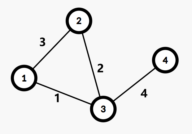
There are clearly two minimum bottleneck paths from 1 to 4: 1-2-3-4 and 1-3-4.

However, edge 1-2 does not occur in any MST.

Applications

Because a minimum bottleneck path need not be unique, problems generally ask for only the maximum edge weight on such a path.

In other words, we need the maximum edge on the relevant MST path.

Binary lifting and heavy-light decomposition can both solve this query, so the details are omitted here.

Kruskal reconstruction tree

Definition

Kruskal processes several edges in increasing order of weight. We use the same order here.

First create $n$ sets, each containing exactly one vertex and having vertex weight $0$ .

Each added edge merges two sets. Create a new vertex with weight equal to the edge weight, make the roots of the two sets its left and right children, and then merge the two sets and the new vertex into one set, with the new vertex as its root.

After $n-1$ rounds, we obtain a binary tree with exactly $n$ leaves, and every non-leaf node has exactly two children. This tree is called the Kruskal reconstruction tree.

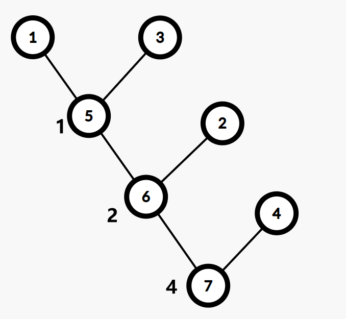
For example:

The Kruskal reconstruction tree for this graph is:

Properties

It is easy to see that the minimum, over all simple paths between two vertices in the original graph, of the maximum edge weight equals the maximum on the simple path between the two vertices in an MST, which equals the weight of the LCA of the two vertices in the Kruskal reconstruction tree.

In other words, for a vertex $x$ , every vertex whose minimum possible maximum edge weight on a simple path is $\leq val$ —call it $y$ —lies in one subtree of the Kruskal reconstruction tree, and these vertices are exactly all the leaves of that subtree.

On the path from $x$ to the root in the Kruskal reconstruction tree, find the shallowest node whose weight is $\leq val$ . Clearly, this is the root of the subtree containing all vertices satisfying the condition.

If we need the maximum, over all simple paths between two vertices in the original graph, of the minimum edge weight, then process Kruskal's edges in decreasing order of weight.

LOJ 137: Minimum bottleneck path (enhanced version)

#include <algorithm>
#include <iostream>

using namespace std;

constexpr int MAX_VAL_RANGE = 280010;

int n, m, log2Values[MAX_VAL_RANGE + 1];

namespace TR {
struct Edge {
  int to, nxt, val;
} e[400010];

int cnt, head[140010];

void addedge(int u, int v, int val = 0) {
  e[++cnt] = Edge{v, head[u], val};
  head[u] = cnt;
}

int val[140010];

namespace LCA {
int sec[280010], cnt;
int pos[140010];
int dpth[140010];

void dfs(int now, int fa) {
  dpth[now] = dpth[fa] + 1;
  sec[++cnt] = now;
  pos[now] = cnt;

  for (int i = head[now]; i; i = e[i].nxt) {
    if (fa != e[i].to) {
      dfs(e[i].to, now);
      sec[++cnt] = now;
    }
  }
}

int dp[280010][20];

void init() {
  dfs(2 * n - 1, 0);
  for (int i = 1; i <= 4 * n; i++) {
    dp[i][0] = sec[i];
  }
  for (int j = 1; j <= 19; j++) {
    for (int i = 1; i + (1 << j) - 1 <= 4 * n; i++) {
      dp[i][j] = dpth[dp[i][j - 1]] < dpth[dp[i + (1 << (j - 1))][j - 1]]
                     ? dp[i][j - 1]
                     : dp[i + (1 << (j - 1))][j - 1];
    }
  }
}

int lca(int x, int y) {
  int l = pos[x], r = pos[y];
  if (l > r) {
    swap(l, r);
  }
  int k = log2Values[r - l + 1];
  return dpth[dp[l][k]] < dpth[dp[r - (1 << k) + 1][k]]
             ? dp[l][k]
             : dp[r - (1 << k) + 1][k];
}
}  // namespace LCA
}  // namespace TR

using TR::addedge;

namespace GR {
struct Edge {
  int u, v, val;

  bool operator<(const Edge &other) const { return val < other.val; }
} e[100010];

int fa[140010];

int find(int x) { return fa[x] == 0 ? x : fa[x] = find(fa[x]); }

void kruskal() {  // Minimum spanning tree
  int tot = 0, cnt = n;
  sort(e + 1, e + m + 1);
  for (int i = 1; i <= m; i++) {
    int fau = find(e[i].u), fav = find(e[i].v);
    if (fau != fav) {
      cnt++;
      fa[fau] = fa[fav] = cnt;
      addedge(fau, cnt);
      addedge(cnt, fau);
      addedge(fav, cnt);
      addedge(cnt, fav);
      TR::val[cnt] = e[i].val;
      tot++;
    }
    if (tot == n - 1) {
      break;
    }
  }
}
}  // namespace GR

int ans;
int A, B, C, P;

int rnd() { return A = (A * B + C) % P; }

void initLog2() {
  for (int i = 2; i <= MAX_VAL_RANGE; i++) {
    log2Values[i] = log2Values[i >> 1] + 1;
  }
}

int main() {
  initLog2();  // Preprocess
  cin >> n >> m;
  for (int i = 1; i <= m; i++) {
    int u, v, val;
    cin >> u >> v >> val;
    GR::e[i] = GR::Edge{u, v, val};
  }
  GR::kruskal();
  TR::LCA::init();
  int Q;
  cin >> Q;
  cin >> A >> B >> C >> P;

  while (Q--) {
    int u = rnd() % n + 1, v = rnd() % n + 1;
    ans += TR::val[TR::LCA::lca(u, v)];
    ans %= 1000000007;
  }
  cout << ans;
  return 0;
}

NOI 2018: Journey home

First preprocess the shortest path from every vertex to the root.

Construct a maximum spanning tree according to altitude. Clearly, the vertices reachable in each query are those whose path to the queried vertex in the maximum spanning tree has minimum edge weight $> p$ .

By the properties of the Kruskal reconstruction tree, these vertices all lie in one subtree and are exactly all its leaves.

In other words, we only need the minimum vertex weight among the leaves of each subtree of the Kruskal reconstruction tree to support subtree queries.

The root of a query can be found using binary lifting on the Kruskal reconstruction tree.

The time complexity is $O((n+m+Q) \log n)$ .