This page mainly introduces algorithms related to the maximum flow problem.
Overview
For the basic concepts of network flow, see Introduction to Network Flow.
Let be a network with a source and a sink. We want to specify a suitable flow on , denoted , to maximize the flow of the entire network (that is, ). This is called the maximum flow problem.
Ford–Fulkerson Augmentation
Ford–Fulkerson augmentation is a general name for a class of algorithms that compute maximum flow. It uses a greedy approach: find augmenting paths and update the maximum flow.
Overview
Given and a flow on , denoted , we make the following definitions.
For an edge , we call the difference between its capacity and flow the residual capacity (Residual Capacity), namely .
The subgraph consisting of all vertices in and all edges whose residual capacity is greater than is called the residual network (Residual Network), namely , where .
Warning
As we will soon mention, flow can be negative, so edges of may not be present in . The introduction of augmentation will explain this in detail below.
In , a path from the source to the sink is called an augmenting path (Augmenting Path). For an augmenting path, we add the same amount of flow to every edge , increasing the flow of the entire network. This process is called augmentation (Augment). Thus, finding a maximum flow can be viewed as superimposing the flows obtained from several augmentations.
In addition, during Ford–Fulkerson augmentation, for every edge we create a reverse edge . We stipulate that . This property can be maintained by introducing flow cancellation during each augmentation: when increases, should decrease by the same amount.
Tip
In implementations of maximum flow algorithms, we often need to access reverse edges quickly. In an adjacency matrix, this is trivial (). However, the mainstream implementation is the more efficient chain forward-star representation. A common technique is to number edges starting from an even number (usually ), and always add the reverse edge immediately after adding an edge, so their numbers are adjacent. Thus, edge and edge are always reverse edges of each other.
Readers encountering this method for the first time may notice a counterintuitive situation: the flow on a reverse edge may be negative. In fact, during Ford–Fulkerson augmentation, the meaningful quantity is the residual capacity , and the absolute value of is irrelevant. We can regard decreasing the flow on the reverse edge as increasing its residual capacity —which is also consistent with the meaning of flow cancellation. Increasing the residual capacity of a reverse edge means that we may next traverse the reverse edge to cancel a previous forward augmentation, representing an operation of “regret”.
The following example may help you understand this process. Suppose is a unit-capacity network, and consider the following process:
- There are multiple augmenting paths in . We choose to perform an augmentation that passes through in that order (as shown in the left figure), increasing the flow by .
- Notice that if we performed the augmentation in the middle figure, the local maximum flow would be not but . However, because the edge entering and the edge leaving exhausted their capacities in the first augmentation, we cannot perform the middle augmentation now. This means our current flow is not optimal, but there may be no other augmenting path locally that uses only edges from the original graph and no reverse edges.
- Now introduce flow cancellation. After the first augmentation, cancellation increases the residual capacity by , which is equivalent to adding a new edge . We can therefore perform another augmentation passing through in that order (the orange path in the right figure). The flows on the undirected edge cancel across the two augmentations, and we are surprised to find that the combined result is actually equivalent to the middle figure.
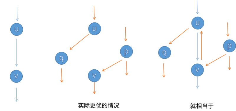
The example above shows that the “cancellation” effect of flow cancellation means we need not worry that we chose augmenting paths in the “wrong” order.
It is easy to see that as long as an augmenting path exists in , augmenting along it increases the total flow; otherwise, the total flow has reached its maximum possible value and the computation is complete. This is the Ford–Fulkerson augmentation process.
Max-Flow Min-Cut Theorem
We have a general understanding of Ford–Fulkerson augmentation, but how can we prove that it is correct? Why is the flow after augmentation ends a maximum flow?
In fact, the correctness of Ford–Fulkerson augmentation is equivalent to the max-flow min-cut theorem (The Maxflow-Mincut Theorem). This theorem states that for any network , its maximum flow and minimum cut always satisfy .
To prove the max-flow min-cut theorem, we first begin with a lemma: for a network , any flow and cut always satisfy . Equality holds if and only if all edges in are saturated and all edges in carry zero flow.
Proof
For equality, the first inequality requires all edges in to carry zero flow, and the second requires all edges in to be saturated. The original lemma follows.
For any network, can the equality conditions above always be satisfied? If the answer is yes, the max-flow min-cut theorem follows. We now prove this.
Proof
Suppose that after one augmentation we obtain a flow such that no augmenting path exists in , that is, in there is no path from to . Let the vertices reachable from form the set , and let .
Clearly, is a cut of , and . Since residual capacities are nonnegative, this also means that for any , we have . We now discuss these edges in two cases, according to whether they exist in the original graph or are reverse edges:
- : in this case, , so ; all edges in are saturated;
- : in this case, ; all edges in carry zero flow.
Therefore, after augmentation stops, the flow satisfies the equality conditions above. By the size relation stated in the lemma, is naturally a maximum flow of , and is a minimum cut of .
It is easy to see that König's theorem is a special case of the max-flow min-cut theorem. In fact, both are related to duality in linear programming.
Time Complexity Analysis
For a network with integer flows, assume trivially that each augmentation has an integer flow. Then an upper bound on the time complexity of Ford–Fulkerson augmentation is , where is the maximum flow on . A single augmentation takes time, and each augmentation increases the total flow, so the number of augmentations cannot exceed .
Different implementations of Ford–Fulkerson augmentation have different time complexities. The more mainstream implementations include Edmonds–Karp, Dinic, SAP, and ISAP, which we introduce separately below.
Edmonds–Karp Algorithm
Algorithm Idea
How do we find an augmenting path in ? When considering a concrete implementation of Ford–Fulkerson augmentation, the most natural approach is to use BFS. Ford–Fulkerson augmentation then becomes the Edmonds–Karp algorithm. Its process is as follows:
-
In , if we can BFS from to , we have found a new augmenting path.
-
For an augmenting path , compute the minimum residual capacity of the edges on , . Add flow to every edge on in an amount of , and cancel flow on each reverse edge, increasing the maximum flow by .
-
Because the flow has changed, we obtain a new . Repeat the process above on the new until no augmenting path exists, at which point the flow no longer increases.
The algorithm above is the Edmonds–Karp algorithm.
Time Complexity Analysis
Next, let us analyze the time complexity of the Edmonds–Karp algorithm.
Clearly, a single BFS augmentation takes time.
The upper bound on the total number of augmentations is . This claim is often falsely proved (or skipped with vague wording) in network-flow materials. We now give a more formal proof1.
Proof of the Upper Bound on the Total Number of Augmentations
First, we introduce a lemma—the shortest-path nondecreasing lemma. Let denote the distance in from vertex to the source (that is, the shortest-path length; the same convention applies below). For one augmentation, let and denote the flow before and after augmentation, respectively. We claim that for every vertex , augmentation always gives . We prove this lemma shortly.
Call an edge with minimum residual capacity on an augmenting path a saturated edge (if several edges attain the minimum, choose any one). If a directed edge is selected as the saturated edge, augmentation empties its residual capacity, causing the saturated edge to disappear, while flow cancellation adds its reverse edge (if the reverse edge did not previously exist), namely and . This analysis shows that for an undirected edge , when augmenting in along , . The residual network then becomes . In , augment along , . By the shortest-path nondecreasing lemma, . Combining these equations gives . In other words, if directed edge is selected as a saturated edge, then compared with the previous time it was selected, the distance from to increases by at least .
The distance from to any vertex cannot exceed . Together with the property above, this shows that each edge is selected as a saturated edge times. Multiplying by the number of edges gives the upper bound on the total number of augmentations.
We now prove the shortest-path nondecreasing lemma, namely . The proof is not difficult, but may be somewhat circuitous, so readers may wish to pause and think carefully.
Proof of the Shortest-Path Nondecreasing Lemma
Consider a contradiction. For one augmentation, suppose that some vertices have a smaller distance to after the augmentation than before it. Let be the one among them with the smallest distance to (that is, ). By the contradiction assumption, is known.
On the shortest path in from to , let be the predecessor of , so .
To ensure that does not violate the property that has the smallest distance, must satisfy .
Adding the two sides of the previous inequality gives . Applying the contradiction assumption, we obtain .
We now discuss the augmentation direction on .
- Suppose . By the BFS property, we have . This conflicts with the inequality above and yields a contradiction.
- Suppose . By the definition of , we know , so this edge must have been created when the current augmentation traversed and generated a reverse edge through cancellation; that is, . This conflicts with the inequality above and yields a contradiction.
Since augmenting along in either direction yields a contradiction, the contradiction assumption is false, and the shortest-path nondecreasing lemma follows.
Multiplying the time complexity of a single BFS augmentation by the upper bound on the number of augmentations, we obtain the Edmonds–Karp time complexity .
Implementation
A possible implementation of the Edmonds–Karp algorithm is as follows.
Reference code
constexpr int MAXN = 250;
constexpr int INF = 0x3f3f3f3f;

struct Edge {
  int from, to, cap, flow;

  Edge(int u, int v, int c, int f) : from(u), to(v), cap(c), flow(f) {}
};

struct EK {
  int n, m;             // n: number of vertices, m: number of edges
  vector<Edge> edges;   // edges: collection of all edges
  vector<int> G[MAXN];  // G: indices in edges of all edges starting at vertex x
  int a[MAXN], p[MAXN];  // a: maximum flow assigned to x by the edge that first reaches x during BFS
                         // p: edge that first reaches x during BFS

  void init(int n) {
    for (int i = 0; i < n; i++) G[i].clear();
    edges.clear();
  }

  void AddEdge(int from, int to, int cap) {
    edges.push_back(Edge(from, to, cap, 0));
    edges.push_back(Edge(to, from, 0, 0));
    m = edges.size();
    G[from].push_back(m - 2);
    G[to].push_back(m - 1);
  }

  int Maxflow(int s, int t) {
    int flow = 0;
    for (;;) {
      memset(a, 0, sizeof(a));
      queue<int> Q;
      Q.push(s);
      a[s] = INF;
      while (!Q.empty()) {
        int x = Q.front();
        Q.pop();
        for (int i = 0; i < G[x].size(); i++) {  // Traverse edges starting at x
          Edge& e = edges[G[x][i]];
          if (!a[e.to] && e.cap > e.flow) {
            p[e.to] = G[x][i];  // G[x][i] is the edge that first reaches e.to
            a[e.to] =
                min(a[x], e.cap - e.flow);  // Assign the flow of the edge that first reaches e.to
            Q.push(e.to);
          }
        }
        if (a[t]) break;  // If the sink has received flow, exit BFS
      }
      if (!a[t])
        break;  // If the sink received no flow, the source and sink are disconnected
      for (int u = t; u != s;
           u = edges[p[u]].from) {  // Trace the s -> t path found by BFS through u
        edges[p[u]].flow += a[t];      // Increase the flow on the path edge
        edges[p[u] ^ 1].flow -= a[t];  // Decrease the flow on the reverse edge
      }
      flow += a[t];
    }
    return flow;
  }
};
Dinic Algorithm
Algorithm Idea
Before augmentation, perform BFS on to build layers, dividing vertices according to the distance from each vertex to the source , denoted . Require flow passing through to move only to a vertex in the next layer; that is, remove outgoing edges from to vertices with equal or smaller layer labels. We call the remaining part of the level graph (Level Graph). Formally, is the level graph of , where .
On , if we find a maximal augmenting flow such that using only it is impossible to increase , then we call a blocking flow of .
Warning
Although above we defined augmentation/augmenting flow only on a single augmenting path, in a broader sense the word “augmentation” can apply not only to the augmenting flow on a single path but also to the union of several augmenting flows—the latter is the sense used in our definition of a blocking flow.
After defining the level graph and blocking flow, the Dinic algorithm proceeds as follows.
- BFS on to construct the level graph .
- DFS on to find a blocking flow .
- Merge into the original flow , namely .
- Repeat the above process until no path from to exists.
The resulting is the maximum flow.
Before analyzing this algorithm's complexity, we need to clarify the process of “using DFS on to find a blocking flow ”. Although BFS layering should be trivial for readers of this page, DFS for a blocking flow requires some technique—we need to introduce current-arc optimization.
During DFS on , if vertex has many incoming and outgoing edges and, whenever receives flow from an incoming edge, it scans the outgoing-edge list to decide which outgoing edge should receive the flow, the local worst-case time complexity at can reach . To avoid this, once we know that edge has been augmented to its limit (edge has no residual capacity or the portion after has already become blocked), there is no need for to try sending flow through outgoing edge again. Accordingly, for each vertex , we maintain the first outgoing edge in the outgoing-edge list of that still needs to be tried. This pointer is conventionally called the current arc, and the technique is called current-arc optimization.
Multi-Path Augmentation
Multi-path augmentation is a constant-factor optimization of the Dinic algorithm. If we find a path from to in the level graph and call it , we need not necessarily start from again to find the next augmenting path; instead, we may start from the last position on that still has residual capacity and search for a branch for another augmentation. Because this is consistent with the backtracking form, the optimization arises naturally in the DFS implementation.
Common Misconception
Perhaps because of the spread of incorrect descriptions in many online resources, a considerable number of contestants like to call current-arc optimization and multi-path augmentation the two optimizations of the Dinic algorithm. In fact, current-arc optimization is part of what ensures the correctness of Dinic's time complexity, whereas multi-path augmentation is merely a constant-factor optimization that does not affect the complexity.
Time Complexity Analysis
After applying current-arc optimization, the time complexity of the Dinic algorithm can be analyzed as follows.
First, we prove that the time complexity of using DFS to find a blocking flow in a single augmentation phase is .
Proof of the Time Complexity of a Single Augmentation Phase
Consider every augmenting path in the blocking flow . Each is obtained on by repeatedly following the current arc, and the number of jumps along each augmenting path is at most .
Each time an augmenting path is found, one saturated edge disappears (its residual capacity becomes zero). For every augmenting path in , let be the set of saturated edges whose residual capacities it clears. Because of the layering property of , after a saturated edge disappears, its reverse edge cannot be traversed by another augmenting path in the same augmentation phase. Therefore, is a subset of .
In addition, for cases where following current arcs is blocked at some position and therefore does not successfully produce an augmenting path, let be the set of final edges on these incomplete paths. Members of are not saturated, so and are disjoint, and is still a subset of .
Every member of is involved in at most jumps (and some jumps are counted repeatedly after multi-path augmentation optimization). Therefore, the total number of jumps in the DFS process is at most .
A Common False Proof
For each vertex, we maintain the next edge that can be augmented, and the current arc changes at most times, so the worst-case time complexity of a single augmentation phase is .
Bug
“The current arc changes at most times” does not imply that “each vertex visits its outgoing edges at most times”. The reason is that visiting the current arc does not necessarily exhaust its residual capacity; vertex may visit the same current arc multiple times.
The number of layers in a level graph obviously cannot exceed . If we can prove that the number of layers strictly increases during augmentation, then the number of augmentation phases of Dinic's algorithm is . We now prove this conclusion2.
Proof of the Monotonicity of the Number of Layers
We introduce a concept from preflow-push algorithms (another class of maximum-flow algorithms)—height labels. To state the proof more conveniently with height labels, let denote the distance in from vertex to the sink , and build layers from the sink rather than the source (there is no essential difference). For one augmentation phase, let and be the flows before and after augmentation. After finding and adding the blocking flow in this phase, let the level graph change from to .
Temporarily, and somewhat informally, define a height label as follows: on a network , let be a function from to the integers ; is a valid height labeling on if and only if holds for every .
Consider , and for each member , we find that for one of two reasons:
- , and its residual capacity was not exhausted during this augmentation phase. By the definition of shortest paths, ;
- , but the blocking flow traversed during this augmentation phase and generated the reverse edge through cancellation. By the definition of the level graph and blocking flow, .
These observations show that is a valid height labeling on , and of course also on and its subgraph , namely the level graph .
Now consider an augmenting path . Starting from the empty path, consider adding vertices one at a time in reverse order along , from to . Suppose has already been added and is being added. After adding , by the definition of the level graph, the value of is greater than by . Meanwhile, because is a height labeling on , may be greater than by , equal to it, or smaller. Therefore, after adding the entire path, we obtain , with equality if and only if for every . If equality does not hold, then —the desired conclusion that the number of layers strictly increases during augmentation. We now prove that equality cannot hold.
Suppose for a contradiction that . We claim that in , the path contains at least one edge ; this edge does not exist in . If no such edge existed, then because , the definitions of the level graph and blocking flow would imply that augmentation in was not complete. To avoid this contradiction, our claim must be true.
Let be an edge satisfying the claim. There are only two possible reasons:
- , but is strict, so by the definition of the level graph, and is added to when the graph is re-layered after augmentation;
- , which means that edge was created when the blocking flow traversed during the current augmentation phase and generated a reverse edge through cancellation, that is, .
In either case, we obtain . Thus the necessary and sufficient condition for equality in cannot be satisfied, contradicting the assumption . The proposition follows.
Another Common False Proof
Suppose for a contradiction that after an augmentation phase the level count is equal to its previous value. Then there should still be at least one augmenting path from to in the level graph with a layer difference of between adjacent vertices. Since this path was not augmented, the augmentation phase has not finished. To avoid the contradiction, the original proposition follows.
[!error]- Bug
“The shortest - path in the new level graph has the same length as before the augmentation phase” does not imply that “the augmentation in the old level graph has not finished”. There is no reason that the two level graphs have the same edge set; the shortest - path in the new level graph may use an edge that did not exist in the old level graph.
Multiplying the single-phase time complexity by the bound on the number of augmentation phases gives the Dinic time complexity .
To make the actual running time of Dinic close to its theoretical upper bound, we would need to construct an input network with special properties. In algorithm competitions, however, network-flow problems usually focus on modeling the original problem as a flow network. Such models generally do not contain the special properties that make Dinic slow; on the contrary, Dinic is highly efficient on most graphs. Therefore, network-flow problems usually have large data ranges, and estimating running time by substituting into is not applicable. Accurate estimation requires contestants to have some experience with Dinic's practical efficiency, so readers should practice more.
Time Complexity Analysis for Special Cases
On some well-behaved graphs, Dinic has a better time complexity.
For a network , if all edge capacities are , that is, for every , then is called a unit-capacity network (Unit Capacity).
In a unit-capacity network, the time complexity of one augmentation phase of Dinic is .
Proof
This is because every augmentation saturates and removes all edges on the augmenting path, so each edge can be augmented only once in a single augmentation phase.
In a unit-capacity network, the number of augmentation phases of Dinic is .
Proof
Build layers centered at the source , let denote the distance in from vertex to the source . In addition, define the set as the layer with index , denoted , and let .
Suppose we have performed augmentation phases. By the pigeonhole principle, there is at least one such that the edge set has size at most . Clearly, is a cut in separating and , and its cut capacity is at most . By the max-flow min-cut theorem, the maximum flow in is at most , meaning that in at most more augmentation phases can be performed. Therefore, the total number of augmentation phases is .
In a unit-capacity network, the number of augmentation phases of Dinic is .
Proof
Suppose we have performed augmentation phases. Since at most half of the layers ( of them) can contain more than vertices, regardless of how the layer sizes are distributed, there is at least one such that two adjacent layers each contain at most vertices, namely and .
To maximize the number of edges between and , assume they form a complete bipartite graph. Then the edge set has size at most . Clearly, is a cut in separating and , and its cut capacity is at most . By the max-flow min-cut theorem, the maximum flow in is at most , meaning that in at most more augmentation phases can be performed. Therefore, the total number of augmentation phases is .
In a unit-capacity network, if every vertex other than the source and sink satisfies or , then the number of augmentation phases of Dinic is . Here, and denote the in-degree and out-degree of vertex , respectively.
Proof
We introduce the following lemma: for a network of this form, any flow can always be decomposed into several unit-flow, vertex-disjoint augmenting paths.
Suppose we have performed augmentation phases. By the definition of the level graph, every new augmenting path now has length at least .
Consider a decomposition of the maximum flow into augmenting paths in . The number of augmenting paths cannot exceed , meaning that at most more augmentation phases can be performed in . Therefore, the total number of augmentation phases is .
In summary, we obtain the following corollaries.
- On a unit-capacity network, the total time complexity of Dinic is .
- On a unit-capacity network, if every vertex other than the source and sink satisfies or , the total time complexity of Dinic is . For maximum bipartite matching, we commonly use the Hopcroft–Karp algorithm, which is in fact a special case of Dinic on a unit-capacity network satisfying the degree restrictions above.
Implementation
Reference code
struct MF {
  struct edge {
    int v, nxt, cap, flow;
  } e[N];

  int fir[N], cnt = 0;

  int n, S, T;
  ll maxflow = 0;
  int dep[N], cur[N];

  void init() {
    memset(fir, -1, sizeof fir);
    cnt = 0;
  }

  void addedge(int u, int v, int w) {
    e[cnt] = {v, fir[u], w, 0};
    fir[u] = cnt++;
    e[cnt] = {u, fir[v], 0, 0};
    fir[v] = cnt++;
  }

  bool bfs() {
    queue<int> q;
    memset(dep, 0, sizeof(int) * (n + 1));

    dep[S] = 1;
    q.push(S);
    while (q.size()) {
      int u = q.front();
      q.pop();
      for (int i = fir[u]; ~i; i = e[i].nxt) {
        int v = e[i].v;
        if ((!dep[v]) && (e[i].cap > e[i].flow)) {
          dep[v] = dep[u] + 1;
          q.push(v);
        }
      }
    }
    return dep[T];
  }

  int dfs(int u, int flow) {
    if ((u == T) || (!flow)) return flow;

    int ret = 0;
    for (int& i = cur[u]; ~i; i = e[i].nxt) {
      int v = e[i].v, d;
      if ((dep[v] == dep[u] + 1) &&
          (d = dfs(v, min(flow - ret, e[i].cap - e[i].flow)))) {
        ret += d;
        e[i].flow += d;
        e[i ^ 1].flow -= d;
        if (ret == flow) return ret;
      }
    }
    return ret;
  }

  void dinic() {
    while (bfs()) {
      memcpy(cur, fir, sizeof(int) * (n + 1));
      maxflow += dfs(S, INF);
    }
  }
} mf;
MPM Algorithm
The MPM (Malhotra, Pramodh-Kumar and Maheshwari) algorithm obtains maximum flow in two ways: a heap-based priority queue with time complexity , or the commonly used BFS solution with time complexity . This section focuses only on the better and simpler algorithm.
The overall structure of the MPM algorithm is similar to Dinic: it runs in phases, and in each phase finds augmenting paths in the layered residual network of . Its main difference from Dinic is how it finds augmenting paths: the path-finding portion of MPM takes only , giving it a better time complexity than Dinic.
MPM considers vertex capacities rather than edge capacities. In the layered network , if the capacity of vertex , denoted , is defined as the smaller of its incoming and outgoing residual capacities, then:
We call a vertex a reference vertex if and only if . For a reference vertex , we can always increase the flow passing through by , making its capacity . This is because is a directed acyclic graph and every vertex in has capacity at least , so there must be a directed path from through to . We simply increase the flow on every edge of this path by . This path is the augmenting path for this phase. BFS can be used to find augmenting paths. After augmentation, all saturated edges can be removed from , because they will not be used again in this phase. Likewise, any vertex other than and with no outgoing or incoming edges can be removed.
Time Complexity Analysis
Each phase of the MPM algorithm takes time, because there are at most iterations (at least the selected reference vertex is deleted), and in each iteration we delete all traversed edges except at most of them. Summing gives . Since the total number of phases is less than , the total running time of MPM is .
Proof that the Number of Phases Is Less Than V
The MPM algorithm ends in fewer than phases. To prove this, we first need to prove two lemmas.
Lemma 1: after each iteration, the distance from to every vertex does not decrease, that is, .
Proof: Fix a phase and a vertex . Consider in any shortest path from to , denoted . The length of is . Note that can contain only backward and forward edges of . If has no backward edge of , then , because is also a path in . Now suppose that has at least one backward edge and its first such edge is . Then (by the first case). The edge does not belong to , so was affected by the augmenting path of the previous iteration. This means . In addition, . From these two equations and , we get . The remaining part of the path can be handled in the same way.
Lemma 2: .
Proof: Lemma 1 gives . Suppose . Note that can contain only backward and forward edges of . This means contains a shortest path that was not blocked by the augmenting path, which is a contradiction.
Implementation
Reference code
struct MPM {
  struct FlowEdge {
    int v, u;
    long long cap, flow;

    FlowEdge() {}

    FlowEdge(int _v, int _u, long long _cap, long long _flow)
        : v(_v), u(_u), cap(_cap), flow(_flow) {}

    FlowEdge(int _v, int _u, long long _cap)
        : v(_v), u(_u), cap(_cap), flow(0ll) {}
  };

  constexpr static long long flow_inf = 1e18;
  vector<FlowEdge> edges;
  vector<char> alive;
  vector<long long> pin, pout;
  vector<list<int>> in, out;
  vector<vector<int>> adj;
  vector<long long> ex;
  int n, m = 0;
  int s, t;
  vector<int> level;
  vector<int> q;
  int qh, qt;

  void resize(int _n) {
    n = _n;
    ex.resize(n);
    q.resize(n);
    pin.resize(n);
    pout.resize(n);
    adj.resize(n);
    level.resize(n);
    in.resize(n);
    out.resize(n);
  }

  MPM() {}

  MPM(int _n, int _s, int _t) {
    resize(_n);
    s = _s;
    t = _t;
  }

  void add_edge(int v, int u, long long cap) {
    edges.push_back(FlowEdge(v, u, cap));
    edges.push_back(FlowEdge(u, v, 0));
    adj[v].push_back(m);
    adj[u].push_back(m + 1);
    m += 2;
  }

  bool bfs() {
    while (qh < qt) {
      int v = q[qh++];
      for (int id : adj[v]) {
        if (edges[id].cap - edges[id].flow < 1) continue;
        if (level[edges[id].u] != -1) continue;
        level[edges[id].u] = level[v] + 1;
        q[qt++] = edges[id].u;
      }
    }
    return level[t] != -1;
  }

  long long pot(int v) { return min(pin[v], pout[v]); }

  void remove_node(int v) {
    for (int i : in[v]) {
      int u = edges[i].v;
      auto it = find(out[u].begin(), out[u].end(), i);
      out[u].erase(it);
      pout[u] -= edges[i].cap - edges[i].flow;
    }
    for (int i : out[v]) {
      int u = edges[i].u;
      auto it = find(in[u].begin(), in[u].end(), i);
      in[u].erase(it);
      pin[u] -= edges[i].cap - edges[i].flow;
    }
  }

  void push(int from, int to, long long f, bool forw) {
    qh = qt = 0;
    ex.assign(n, 0);
    ex[from] = f;
    q[qt++] = from;
    while (qh < qt) {
      int v = q[qh++];
      if (v == to) break;
      long long must = ex[v];
      auto it = forw ? out[v].begin() : in[v].begin();
      while (true) {
        int u = forw ? edges[*it].u : edges[*it].v;
        long long pushed = min(must, edges[*it].cap - edges[*it].flow);
        if (pushed == 0) break;
        if (forw) {
          pout[v] -= pushed;
          pin[u] -= pushed;
        } else {
          pin[v] -= pushed;
          pout[u] -= pushed;
        }
        if (ex[u] == 0) q[qt++] = u;
        ex[u] += pushed;
        edges[*it].flow += pushed;
        edges[(*it) ^ 1].flow -= pushed;
        must -= pushed;
        if (edges[*it].cap - edges[*it].flow == 0) {
          auto jt = it;
          ++jt;
          if (forw) {
            in[u].erase(find(in[u].begin(), in[u].end(), *it));
            out[v].erase(it);
          } else {
            out[u].erase(find(out[u].begin(), out[u].end(), *it));
            in[v].erase(it);
          }
          it = jt;
        } else
          break;
        if (!must) break;
      }
    }
  }

  long long flow() {
    long long ans = 0;
    while (true) {
      pin.assign(n, 0);
      pout.assign(n, 0);
      level.assign(n, -1);
      alive.assign(n, true);
      level[s] = 0;
      qh = 0;
      qt = 1;
      q[0] = s;
      if (!bfs()) break;
      for (int i = 0; i < n; i++) {
        out[i].clear();
        in[i].clear();
      }
      for (int i = 0; i < m; i++) {
        if (edges[i].cap - edges[i].flow == 0) continue;
        int v = edges[i].v, u = edges[i].u;
        if (level[v] + 1 == level[u] && (level[u] < level[t] || u == t)) {
          in[u].push_back(i);
          out[v].push_back(i);
          pin[u] += edges[i].cap - edges[i].flow;
          pout[v] += edges[i].cap - edges[i].flow;
        }
      }
      pin[s] = pout[t] = flow_inf;
      while (true) {
        int v = -1;
        for (int i = 0; i < n; i++) {
          if (!alive[i]) continue;
          if (v == -1 || pot(i) < pot(v)) v = i;
        }
        if (v == -1) break;
        if (pot(v) == 0) {
          alive[v] = false;
          remove_node(v);
          continue;
        }
        long long f = pot(v);
        ans += f;
        push(v, s, f, false);
        push(v, t, f, true);
        alive[v] = false;
        remove_node(v);
      }
    }
    return ans;
  }
};
ISAP
In the Dinic algorithm, we run BFS to build layers after finding augmenting paths each time. Is there a more efficient method?
The answer is the ISAP algorithm introduced below.
Process
As in Dinic, we first run BFS to layer the vertices, but unlike Dinic, we run BFS on the reverse graph, from to .
After the layering process, we use DFS to find augmenting paths.
The augmentation process is similar to Dinic: we only augment to vertices whose layer is less than the current vertex's layer.
Unlike Dinic, we do not rerun BFS to layer the graph. Instead, we complete the relayering during augmentation.
Specifically, let the layer of vertex be . After finishing augmentation at vertex , we traverse all outgoing edges of in the residual network and find the outgoing vertex with the smallest layer. We then set . In particular, if has no outgoing edge in the residual network, set .
It is easy to see that when , no augmenting path exists in the graph, so the algorithm can terminate.
As in Dinic, ISAP also has current-arc optimization.
For layer , we record the number of vertices as . Whenever a vertex's layer changes from to , we update the array accordingly. If after the update , a gap has appeared in the graph and no augmenting path can be found; the algorithm can terminate immediately (in the implementation, set directly to ). This optimization is called GAP optimization.
Implementation
Reference code
struct Edge {
  int from, to, cap, flow;

  Edge(int u, int v, int c, int f) : from(u), to(v), cap(c), flow(f) {}
};

bool operator<(const Edge& a, const Edge& b) {
  return a.from < b.from || (a.from == b.from && a.to < b.to);
}

struct ISAP {
  int n, m, s, t;
  vector<Edge> edges;
  vector<int> G[MAXN];
  bool vis[MAXN];
  int d[MAXN];
  int cur[MAXN];
  int p[MAXN];
  int num[MAXN];

  void AddEdge(int from, int to, int cap) {
    edges.push_back(Edge(from, to, cap, 0));
    edges.push_back(Edge(to, from, 0, 0));
    m = edges.size();
    G[from].push_back(m - 2);
    G[to].push_back(m - 1);
  }

  bool BFS() {
    memset(vis, 0, sizeof(vis));
    queue<int> Q;
    Q.push(t);
    vis[t] = true;
    d[t] = 0;
    while (!Q.empty()) {
      int x = Q.front();
      Q.pop();
      for (int i = 0; i < G[x].size(); i++) {
        Edge& e = edges[G[x][i] ^ 1];
        if (!vis[e.from] && e.cap > e.flow) {
          vis[e.from] = true;
          d[e.from] = d[x] + 1;
          Q.push(e.from);
        }
      }
    }
    return vis[s];
  }

  void init(int n) {
    this->n = n;
    for (int i = 0; i < n; i++) G[i].clear();
    edges.clear();
  }

  int Augment() {
    int x = t, a = INF;
    while (x != s) {
      Edge& e = edges[p[x]];
      a = min(a, e.cap - e.flow);
      x = edges[p[x]].from;
    }
    x = t;
    while (x != s) {
      edges[p[x]].flow += a;
      edges[p[x] ^ 1].flow -= a;
      x = edges[p[x]].from;
    }
    return a;
  }

  int Maxflow(int s, int t) {
    this->s = s;
    this->t = t;
    int flow = 0;
    BFS();
    memset(num, 0, sizeof(num));
    for (int i = 0; i < n; i++) num[d[i]]++;
    int x = s;
    memset(cur, 0, sizeof(cur));
    while (d[s] < n) {
      if (x == t) {
        flow += Augment();
        x = s;
      }
      int ok = 0;
      for (int i = cur[x]; i < G[x].size(); i++) {
        Edge& e = edges[G[x][i]];
        if (e.cap > e.flow && d[x] == d[e.to] + 1) {
          ok = 1;
          p[e.to] = G[x][i];
          cur[x] = i;
          x = e.to;
          break;
        }
      }
      if (!ok) {
        int m = n - 1;
        for (int i = 0; i < G[x].size(); i++) {
          Edge& e = edges[G[x][i]];
          if (e.cap > e.flow) m = min(m, d[e.to]);
        }
        if (--num[d[x]] == 0) break;
        num[d[x] = m + 1]++;
        cur[x] = 0;
        if (x != s) x = edges[p[x]].from;
      }
    }
    return flow;
  }
};
Push-Relabel Algorithm
This method ignores flow conservation during the computation and updates one vertex at a time to solve maximum flow.
General Preflow-Push Algorithm
We first introduce the main idea of the preflow-push algorithm and a feasible brute-force implementation.
The preflow-push algorithm solves maximum flow by repeatedly updating individual vertices until no vertex needs to be updated.
The flow function maintained during the algorithm does not necessarily satisfy flow conservation. For a vertex , we allow the flow entering it to exceed the flow leaving it; the excess is called the excess flow :
If , vertex is called overflowing3. Note that when we mention an overflowing vertex, we exclude and .
The preflow-push algorithm maintains the height of each vertex and stipulates that an overflowing vertex may push excess flow only to a vertex whose height is less than ; if has no adjacent vertex whose height is less than , modify the height of (relabel it).
Height Function4
More precisely, preflow-push maintains the following mapping :
We call a height function of the residual network .
Lemma 1: If has height function , then for any two vertices , if , is not an edge of .
The algorithm performs push operations only on edges satisfying .
Push
Applicable condition: vertex is overflowing, and there exists vertex ; the push operation applies to .
We then push as much excess flow as possible from to . During the push, we care only about the smaller of the excess flow and ; whether overflows is irrelevant.
If becomes saturated after the push, remove it from the residual network.
Relabel
Applicable condition: if vertex is overflowing and , then the relabel operation applies to .
Then update to .
Initialization
The above saturates every and raises , making , because and the edge is already saturated, so there is no need to keep it in the residual network. It also initializes to the negative of .
Process
We scan the entire graph repeatedly; whenever there is a vertex satisfying the conditions for a push or relabel operation, we perform the corresponding operation.
As shown, the number is displayed in the middle of each vertex, the height value at the lower left, and the excess flow at the lower right. The depth of the vertex color also represents its height. Edge weights represent , and green edges satisfy ; they are edges of the residual network .
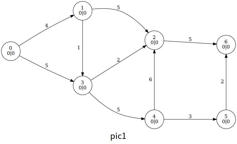
Let us briefly review the process of the entire algorithm. Here the author uses a brute-force algorithm that scans for overflowing vertices and updates one whenever it finds one.
The final result
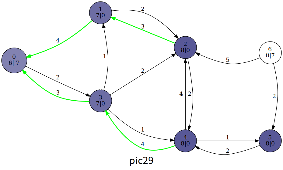
We can see that in the end, some excess flow has returned to , and no vertex other than the source and sink is overflowing. The flow function now satisfies flow conservation and is a maximum flow; its value is .
However, the paper5 points out that processing only overflowing vertices with height less than still gives the correct maximum-flow value. In that case, though, the preflow at the end of the algorithm does not yet satisfy the properties of a flow function, so the actual flow on each edge cannot be determined.
Implementation
Core code
constexpr int N = 1e4 + 4, M = 1e5 + 5, INF = 0x3f3f3f3f;
int n, m, s, t, maxflow, tot;
int ht[N], ex[N];

void init() {  // Initialization
  for (int i = h[s]; i; i = e[i].nex) {
    const int &v = e[i].t;
    ex[v] = e[i].v, ex[s] -= ex[v], e[i ^ 1].v = e[i].v, e[i].v = 0;
  }
  ht[s] = n;
}

bool push(int ed) {
  const int &u = e[ed ^ 1].t, &v = e[ed].t;
  int flow = min(ex[u], e[ed].v);
  ex[u] -= flow, ex[v] += flow, e[ed].v -= flow, e[ed ^ 1].v += flow;
  return ex[u];  // Return 1 if u is still overflowing
}

void relabel(int u) {
  ht[u] = INF;
  for (int i = h[u]; i; i = e[i].nex)
    if (e[i].v) ht[u] = min(ht[u], ht[e[i].t]);
  ++ht[u];
}
HLPP Algorithm
The Highest Label Preflow Push algorithm prioritizes the overflowing vertex with the greatest height whenever it selects a vertex in the general preflow-push algorithm above. Its time complexity is .
Process
Specifically, the HLPP algorithm proceeds as follows:
- Initialize based on the preflow-push algorithm.
- Select the highest-height overflowing vertex , and push along every edge through which it can push.
- If is still overflowing, relabel it and return to step 2.
- If there is no overflowing vertex, terminate the algorithm.
A paper testing the practical performance of maximum-flow algorithms6 shows that preflow-based algorithms actually spend a considerable portion of their time on relabeling. We introduce below two optimizations from the paper7 that can significantly reduce the number of relabel operations.
BFS Optimization
The upper bound of HLPP is , but it is relatively tight in practice. We can optimize the initial heights. Specifically, initialize to the shortest distance from to ; in particular, .
During BFS, we also check graph connectivity and rule out cases with no solution.
GAP Optimization
The push condition in HLPP is . If at some point in the algorithm there is a such that the number of vertices with is , then vertices with can never push excess flow to and can only send it back to . We therefore immediately raise their heights to at least , so that they can push back to as quickly as possible and reduce relabel operations.
The implementation below follows the method in paper6 and uses buckets B, where B[i] records all overflowing vertices currently at height . It includes the two optimizations above and processes only overflowing vertices with height less than .
It is worth noting that the buckets in paper6 use stacks based on linked lists, whereas the default container for stack in the STL is deque. Simple tests show little difference in the actual running efficiency of vector, deque, and list for this problem.
Implementation
LuoguP4722 [Template] Maximum Flow, Enhanced Version/Preflow-Push
#include <cstdio>
#include <cstring>
#include <queue>
#include <stack>
using namespace std;
constexpr int N = 1200, M = 120000, INF = 0x3f3f3f3f;
int n, m, s, t;

struct qxx {
  int nex, t;
  long long v;
};

qxx e[M * 2 + 1];
int h[N + 1], cnt = 1;

void add_path(int f, int t, long long v) {
  e[++cnt] = qxx{h[f], t, v}, h[f] = cnt;
}

void add_flow(int f, int t, long long v) {
  add_path(f, t, v);
  add_path(t, f, 0);
}

int ht[N + 1];        // height;
long long ex[N + 1];  // excess flow;
int gap[N];           // GAP optimization. gap[i] is the number of vertices at height i
stack<int> B[N];      // Bucket B[i] stores all v with ht[v]==i
int level = 0;        // maximum height of an overflowing vertex

int push(int u) {      // Push as much excess flow as possible through usable edges
  bool init = u == s;  // whether this is initialization
  for (int i = h[u]; i; i = e[i].nex) {
    const int &v = e[i].t;
    const long long &w = e[i].v;
    // During initialization, do not require a height difference of 1
    if (!w || (init == false && ht[u] != ht[v] + 1) || ht[v] == INF) continue;
    long long k = init ? w : min(w, ex[u]);
    // Take the minimum of residual capacity and excess flow; initialization may make the source's excess negative.
    if (v != s && v != t && !ex[v]) B[ht[v]].push(v), level = max(level, ht[v]);
    ex[u] -= k, ex[v] += k, e[i].v -= k, e[i ^ 1].v += k;  // push
    if (!ex[u]) return 0;  // Return if all flow has been pushed
  }
  return 1;
}

void relabel(int u) {  // Relabel (height)
  ht[u] = INF;
  for (int i = h[u]; i; i = e[i].nex)
    if (e[i].v) ht[u] = min(ht[u], ht[e[i].t]);
  if (++ht[u] < n) {  // Process only vertices with height less than n
    B[ht[u]].push(u);
    level = max(level, ht[u]);
    ++gap[ht[u]];  // New height; update GAP
  }
}

bool bfs_init() {
  memset(ht, 0x3f, sizeof(ht));
  queue<int> q;
  q.push(t), ht[t] = 0;
  while (q.size()) {  // Reverse BFS; enqueue an unvisited vertex
    int u = q.front();
    q.pop();
    for (int i = h[u]; i; i = e[i].nex) {
      const int &v = e[i].t;
      if (e[i ^ 1].v && ht[v] > ht[u] + 1) ht[v] = ht[u] + 1, q.push(v);
    }
  }
  return ht[s] != INF;  // Return 0 if the graph is disconnected
}

// Select one of the vertices at the current maximum height; return 0 if no overflowing vertex remains
int select() {
  while (level > -1 && B[level].size() == 0) level--;
  return level == -1 ? 0 : B[level].top();
}

long long hlpp() {            // Return the maximum flow
  if (!bfs_init()) return 0;  // The graph is disconnected
  memset(gap, 0, sizeof(gap));
  for (int i = 1; i <= n; i++)
    if (ht[i] != INF) gap[ht[i]]++;  // Initialize GAP
  ht[s] = n;
  push(s);  // Initialize the preflow
  int u;
  while ((u = select())) {
    B[level].pop();
    if (push(u)) {  // Still overflowing
      if (!--gap[ht[u]])
        for (int i = 1; i <= n; i++)
          if (i != s && ht[i] > ht[u] && ht[i] < n + 1)
            ht[i] = n + 1;  // Vertices relabeled to n+1 here are not overflowing
      relabel(u);
    }
  }
  return ex[t];
}

int main() {
  scanf("%d%d%d%d", &n, &m, &s, &t);
  for (int i = 1, u, v, w; i <= m; i++) {
    scanf("%d%d%d", &u, &v, &w);
    add_flow(u, v, w);
  }
  printf("%lld", hlpp());
  return 0;
}
Feel the execution process
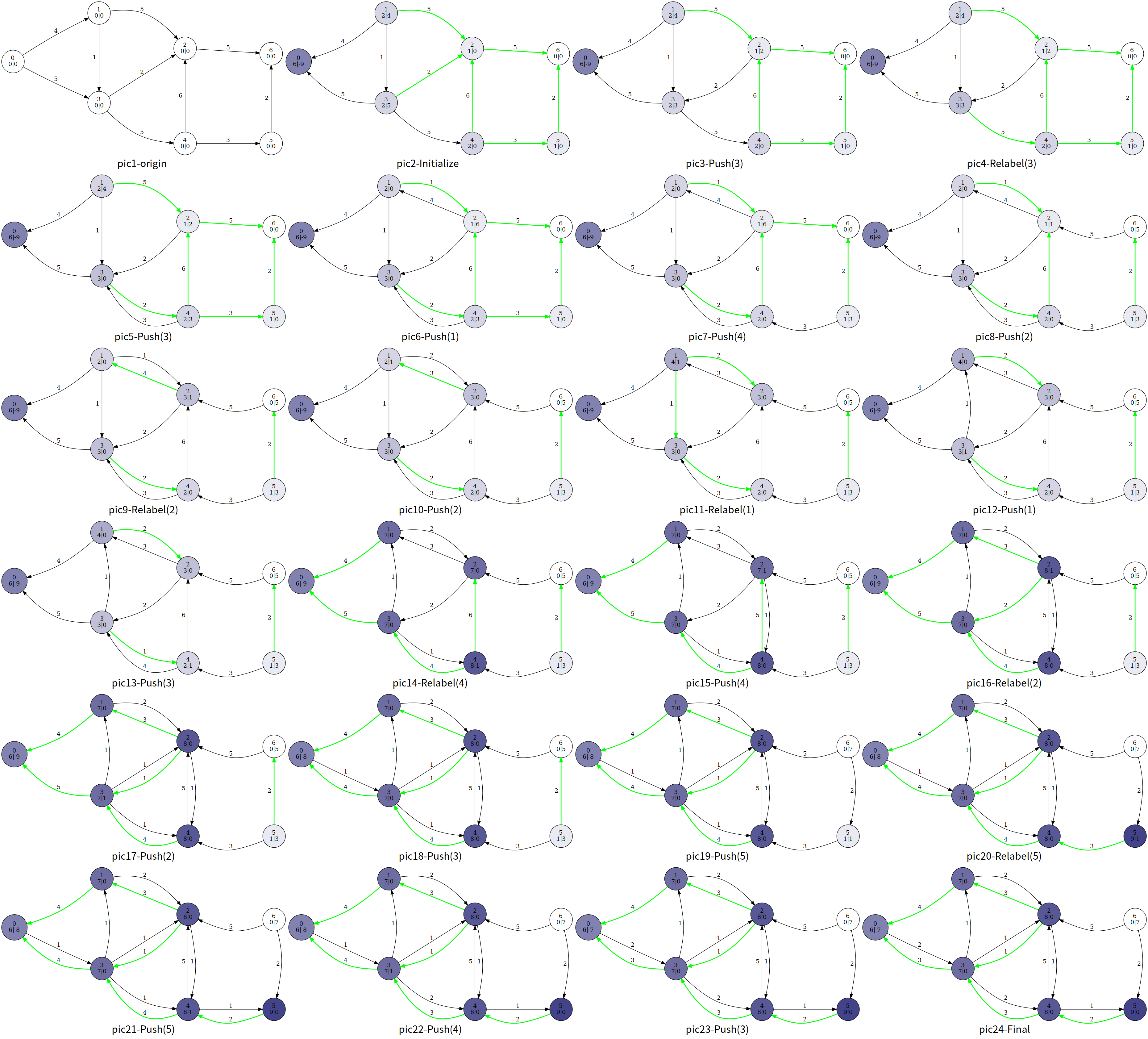
Relabel(4) is performed from pic13 to pic14, together with GAP optimization.
Footnotes
Footnotes
-
http://pisces.ck.tp.edu.tw/~peng/index.php?action=showfile&file=f6cdf7ef750d7dc79c7d599b942acbaaee86a2e3e ↩
-
https://people.orie.cornell.edu/dpw/orie633/LectureNotes/lecture9.pdf ↩
-
English-language literature usually calls it “active”. ↩
-
In English-language literature, the height of a vertex is usually called a “distance label”. The term “height” used here comes from the relevant chapter of Introduction to Algorithms. You can find the reason for this choice in footnote P432 of the Chinese edition of Introduction to Algorithms (3rd edition) published by China Machine Press. ↩
-
Cherkassky B V, Goldberg A V. On implementing push-relabel method for the maximum flow problem[C]//International Conference on Integer Programming and Combinatorial Optimization. Springer, Berlin, Heidelberg, 1995: 157-171. ↩
-
Ahuja R K, Kodialam M, Mishra A K, et al. Computational investigations of maximum flow algorithms[J]. European Journal of Operational Research, 1997, 97(3): 509-542. ↩ ↩2 ↩3
-
Derigs U, Meier W. Implementing Goldberg's max-flow-algorithm—A computational investigation[J]. Zeitschrift für Operations Research, 1989, 33(6): 383-403. ↩