AIOJ

Introduction

A bipartite graph, also called a bigraph, is a graph with a special structure. Its vertex set can be partitioned into two disjoint subsets such that every edge connects a pair of vertices from the two sets and no edge connects vertices within the same set.

Thanks to this simple structure, bipartite graphs not only have many elegant properties, but are also widely used to model real-world scenarios such as task assignment, recommendation systems, and matching markets. Many optimization problems that are difficult on general graphs can be solved efficiently and exactly on bipartite graphs.

Definition

If the vertex set $G=(V,E)$ of a graph $V$ can be divided into two disjoint subsets $X$ and $Y$ such that the two endpoints of every edge $e\in E$ belong to $X$ and $Y$ , respectively, then $G$ is called a bipartite graph. The sets $X$ and $Y$ are often called its two parts, or the left and right parts of the bipartite graph, respectively. When the two parts $X$ and $Y$ of a bipartite graph are known, the bipartite graph $(X, Y, E)$ can also be represented by the triple $G$ .

A typical bipartite graph is shown below.

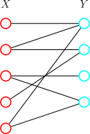
Trees, even cycles, and grid graphs are common examples of bipartite graphs.

Characterizations

A bipartite graph can equivalently be defined by the following properties:

The graph $G$ is 2-colorable. That is, all vertices can be colored with at most two colors so that adjacent vertices have different colors.
The graph $G$ contains no cycle of odd length.

It is clear that the first property is equivalent to the definition of a bipartite graph: simply color the two parts of the bipartite graph with different colors.

The second property is slightly more complicated. Consider trying to color $G$ with two colors. Since coloring in different connected components does not interfere, it suffices to consider the connected components one by one. Choose any vertex $s$ in a connected component, perform DFS, and record the distance from $v$ to each vertex $s$ in the component. Starting from $s$ , induction on the DFS tree shows that if a valid coloring exists, the two colors must be assigned according to the parity of the distance from each vertex $v$ to the starting vertex $s$ .

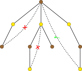
Now consider the edges outside the spanning tree. If the endpoints of every such non-tree edge have different colors, the current coloring is valid; otherwise, no valid coloring exists. Furthermore, two vertices have different colors if and only if their distances from the tree root $s$ have different parity, which is equivalent to saying that adding the non-tree edge creates an even rather than an odd cycle. Therefore, if there is no odd cycle, these non-tree edges must connect vertices of different colors, and the entire graph can be colored with two colors. Thus the graph must be bipartite.

Recognition

To determine whether a graph is bipartite, it suffices to use the equivalent characterizations above and try to color it. We can traverse the graph using DFS or BFS. If an odd cycle is found, meaning that coloring is impossible, the graph is not bipartite; otherwise, it is bipartite.

The process is as follows:

Traverse the vertices. If an uncolored vertex is found, a new connected component has been found.
Assign any color to the vertex and use it as the starting point for DFS or BFS, attempting to color the connected component.
When traversing adjacent vertices, if an already colored vertex is found, check whether its color is the same as the current vertex. If so, the graph is not bipartite and we can return immediately; otherwise, continue traversing.
If an uncolored vertex is found, color it with the color opposite to that of the current vertex.

The reference code is as follows:

Reference code

int n;
std::vector<std::vector<int>> gr;
std::vector<int> colors, vis;

// Depth-first search to color vertices.
bool dfs(int cr) {
  vis[cr] = true;
  for (int nt : gr[cr]) {
    if (vis[nt]) {
      if (colors[cr] == colors[nt]) return false;
    } else {
      colors[nt] = colors[cr] ^ 1;
      if (!dfs(nt)) return false;
    }
  }
  return true;
}

// Check whether the graph GR is bipartite.
// If so, the vector COLORS will store a feasible coloring.
bool check_bipartite() {
  for (int i = 1; i <= n; ++i) {
    // Check connected components one by one.
    if (!vis[i]) {
      colors[i] = 0;
      if (!dfs(i)) return false;
    }
  }
  return true;
}

The time complexity is $O(|V|+|E|)$ .

Applications

Because of their simple structure, many graph optimization problems can be solved efficiently on bipartite graphs. See the corresponding main articles for details.

Bipartite graph

Introduction

Definition

Characterizations

Recognition

Applications