AIOJ

Introduction

Before reading the following material, be sure to understand the fundamentals in Graph Theory Concepts.

A directed graph G is strongly connected if every pair of vertices in G is connected.

A strongly connected component (SCC) is a maximal strongly connected subgraph.

This page explains how to find strongly connected components.

Tarjan's Algorithm

Introduction

Robert E. Tarjan (1948–), born in Pomona, California, is an American computer scientist.

Tarjan invented many algorithms and data structures. Many of the algorithms he invented are named after him, sometimes making different algorithms confusingly similar. Examples include Tarjan's algorithms for finding various connected components and Tarjan's algorithm for finding the LCA (Lowest Common Ancestor). Disjoint-set union, Splay, and Top Tree were also invented by Tarjan.

Here we introduce Tarjan's algorithm for finding strongly connected components in a directed graph.

DFS Spanning Forest

Before introducing the algorithm, let us first understand the DFS spanning tree, using the following directed graph as an example:

DFS spanning tree

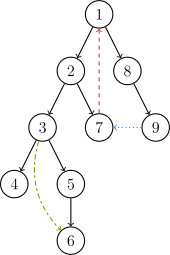
When running DFS on a directed graph $G$ , edge directions may prevent all vertices from being reached from a single vertex. Therefore, we must traverse the entire vertex set: start a new DFS from every vertex that has not yet been visited. During each completed DFS starting from a particular vertex, the tree edges it traverses (see below) form a tree called a DFS spanning tree. After all vertices have been visited, the collection of these DFS spanning trees forms the directed graph's DFS spanning forest.

The precise structure of the spanning tree (and forest), as well as the edge classification below, depends on the choice of DFS starting vertex and the order in which adjacent vertices are visited.

The edges of a directed graph $G$ can be divided into four categories:

Tree edge: shown in black in the diagram; a tree edge is formed each time the search finds a vertex that has not yet been visited. All adjacent tree edges form a DFS spanning tree.
Back edge: also called a return edge, shown in red (that is, $7 \rightarrow 1$ ); a non-tree edge from a vertex to one of its ancestors during the search.
Forward edge: shown in green (that is, $3 \rightarrow 6$ ); a non-tree edge from a vertex to a descendant in its subtree during the search.
Cross edge: shown in blue (that is, $9 \rightarrow 7$ ); an edge from a vertex to a visited vertex that is neither an ancestor nor a descendant, and therefore belongs to none of the preceding three categories.

We now consider the relationship between DFS spanning trees and strongly connected components.

If vertex $u$ is the first vertex of a strongly connected component encountered in the search tree, all other vertices in that component must lie in the subtree rooted at $u$ in the search tree. Vertex $u$ is called the root of that strongly connected component.

Proof by contradiction: suppose a vertex $v$ belongs to the strongly connected component but is not in the subtree rooted at $u$ . Then the path from $u$ to $v$ must contain an edge leaving the subtree. Such an edge can only be a cross edge or a back edge, but both kinds require their destination to have already been visited, contradicting the fact that $v$ is not in the subtree rooted at $u$ . Thus the claim follows.

Tarjan's Algorithm for Strongly Connected Components

Tarjan's algorithm is based on depth-first search. We regard each connected component as a subtree of the search tree and maintain a stack during the search, pushing each not-yet-processed node of the search tree onto it.

For every vertex $u$ , Tarjan's algorithm maintains the following variables:

$\textit{dfn}_u$ : the order in which vertex $u$ is visited during depth-first search.
$\textit{low}_u$ : the earliest vertex still on the stack that can be reached by backtracking from the subtree of $u$ . Let $\textit{Subtree}_u$ denote the subtree rooted at $u$ . $\textit{low}_u$ is the minimum $\textit{dfn}$ among the following vertices: vertices in $\textit{Subtree}_u$ , and vertices reachable from $\textit{Subtree}_u$ through an edge outside the search tree.

Every vertex in a node's subtree has a larger dfn than that node.

Along a path from the root, dfn values increase strictly and low values are nondecreasing.

Search all vertices in the order specified by depth-first search, maintain each vertex's dfn and low, and push every visited vertex onto the stack. Whenever a strongly connected component is found, pop from the stack as many vertices as the component contains. For a vertex $u$ and an adjacent vertex $v$ ( $v$ is not the parent of $u$ ), consider three cases:

$v$ has not been visited: continue the depth-first search from $v$ . During backtracking, use $\textit{low}_v$ to update $\textit{low}_u$ . Because there is a direct path from $u$ to $v$ , every vertex still on the stack that $v$ can reach by backtracking can also be reached by $u$ .
$v$ has been visited and is still on the stack: by the definition of low, use $\textit{dfn}_v$ to update $\textit{low}_u$ .
$v$ has been visited and is no longer on the stack: this means that the search of $v$ and the component containing it are complete, so no operation is needed.

The algorithm above can be written as the following pseudocode:

Implementation

TARJAN_SEARCH(int u)
    vis[u]=true
    low[u]=dfn[u]=++dfncnt
    push u to the stack
    for each (u,v) then do
        if v hasn't been searched then
            TARJAN_SEARCH(v) // search
            low[u]=min(low[u],low[v]) // backtrack
        else if v has been in the stack then
            low[u]=min(low[u],dfn[v])

For a connected-component graph, it is easy to see that there is exactly one $u$ in the connected graph satisfying $\textit{dfn}_u=\textit{low}_u$ . This vertex must be the first vertex of the component visited during the depth-first traversal: its dfn and low values are the smallest and cannot be affected by other vertices in the component.

Therefore, during backtracking, check whether $\textit{dfn}_u=\textit{low}_u$ . If so, $u$ and all vertices above it on the stack form an SCC.

Implementation

C++

int dfn[N], low[N], dfncnt, s[N], in_stack[N], tp;
int scc[N], sc;  // ID of the SCC containing vertex i
int sz[N];       // size of SCC i

void tarjan(int u) {
  low[u] = dfn[u] = ++dfncnt, s[++tp] = u, in_stack[u] = 1;
  for (int i = h[u]; i; i = e[i].nex) {
    const int &v = e[i].t;
    if (!dfn[v]) {
      tarjan(v);
      low[u] = min(low[u], low[v]);
    } else if (in_stack[v]) {
      low[u] = min(low[u], dfn[v]);
    }
  }
  if (dfn[u] == low[u]) {
    ++sc;
    do {
      scc[s[tp]] = sc;
      sz[sc]++;
      in_stack[s[tp]] = 0;
    } while (s[tp--] != u);
  }
}

Python

dfn = [0] * N
low = [0] * N
dfncnt = 0
s = [0] * N
in_stack = [0] * N
tp = 0
scc = [0] * N
sc = 0  # ID of the SCC containing vertex i
sz = [0] * N  # size of SCC i

def tarjan(u):
    low[u] = dfn[u] = dfncnt
    s[tp] = u
    in_stack[u] = 1
    dfncnt = dfncnt + 1
    tp = tp + 1
    i = h[u]
    while i:
        v = e[i].t
        if dfn[v] == False:
            tarjan(v)
            low[u] = min(low[u], low[v])
        elif in_stack[v]:
            low[u] = min(low[u], dfn[v])
        i = e[i].nex
    if dfn[u] == low[u]:
        sc = sc + 1
        while s[tp] != u:
            scc[s[tp]] = sc
            sz[sc] = sz[sc] + 1
            in_stack[s[tp]] = 0
            tp = tp - 1
        scc[s[tp]] = sc
        sz[sc] = sz[sc] + 1
        in_stack[s[tp]] = 0
        tp = tp - 1

The time complexity is $O(n + m)$ .

The Relationship Between Component Labels and Topological Order

During processing, Tarjan's algorithm actually discovers strongly connected components in a kind of reverse topological order. This is because depth-first search first finishes vertices with no outgoing edges, which is the opposite of the topological-sorting process.

If we contract every strongly connected component in the graph into a single vertex, then perform a topological sort in the DAG formed by the contracted vertices, the resulting order is the reverse of the label order assigned to the components by Tarjan's algorithm.

Therefore, in the contracted DAG, the labels of strongly connected components (after contraction) are in reverse topological order. Note, however, that this statement holds only when considering the dependencies between strongly connected components (that is, directed edges from one component to another). The vertices inside a single strongly connected component contain cycles, so their internal order does not satisfy the definition of a topological order.

Kosaraju's Algorithm

Introduction

Kosaraju's algorithm was first proposed in 1978 by S. Rao Kosaraju in an unpublished paper, but Micha Sharir was the first to publish it.

Process

The algorithm uses two simple DFS passes:

In the first DFS, choose any vertex as the starting point, visit every unvisited vertex, and assign vertices numbers before backtracking; this is a postorder traversal.

In the second DFS, reverse the graph and start from the vertex with the largest label. The set of vertices reached is a strongly connected component. For every still-unvisited vertex, choose the one with the largest label and repeat.

After the two DFS passes, the strongly connected components have been found. Kosaraju's algorithm has time complexity $O(n+m)$ .

Implementation

C++

// g is the original graph; g2 is the reversed graph

void dfs1(int u) {
  vis[u] = true;
  for (int v : g[u])
    if (!vis[v]) dfs1(v);
  s.push_back(u);
}

void dfs2(int u) {
  color[u] = sccCnt;
  for (int v : g2[u])
    if (!color[v]) dfs2(v);
}

void kosaraju() {
  sccCnt = 0;
  for (int i = 1; i <= n; ++i)
    if (!vis[i]) dfs1(i);
  for (int i = n; i >= 1; --i)
    if (!color[s[i]]) {
      ++sccCnt;
      dfs2(s[i]);
    }
}

Python

def dfs1(u):
    vis[u] = True
    for v in g[u]:
        if vis[v] == False:
            dfs1(v)
    s.append(u)

def dfs2(u):
    color[u] = sccCnt
    for v in g2[u]:
        if color[v] == False:
            dfs2(v)

def kosaraju(u):
    sccCnt = 0
    for i in range(1, n + 1):
        if vis[i] == False:
            dfs1(i)
    for i in range(n, 0, -1):
        if color[s[i]] == False:
            sccCnt = sccCnt + 1
            dfs2(s[i])

Garbow's Algorithm

Process

Garbow's algorithm is another implementation of Tarjan's algorithm. Tarjan uses dfn and low to compute the roots of strongly connected components; Garbow maintains one node stack and uses a second stack to determine when to pop from the first stack the nodes belonging to the same strongly connected component. During the DFS starting at node $w$ , when a path shows that a group of nodes belongs to the same strongly connected component, pop nodes from the second stack while the top node's visit time is greater than the visit time of the root $w$ , leaving only the root $w$ . Every node popped in this process belongs to the same strongly connected component.

When backtracking to a node $w$ , if it is at the top of the second stack, then it is the starting node of a strongly connected component. The nodes visited after this node belong to the same component, so pop them from the first stack to form the component.

Implementation

C++

int garbow(int u) {
  stack1[++p1] = u;
  stack2[++p2] = u;
  low[u] = ++dfs_clock;
  for (int i = head[u]; i; i = e[i].next) {
    int v = e[i].to;
    if (!low[v])
      garbow(v);
    else if (!sccno[v])
      while (low[stack2[p2]] > low[v]) p2--;
  }
  if (stack2[p2] == u) {
    p2--;
    scc_cnt++;
    do {
      sccno[stack1[p1]] = scc_cnt;
      // all_scc[scc_cnt] ++;
    } while (stack1[p1--] != u);
  }
  return 0;
}

void find_scc(int n) {
  dfs_clock = scc_cnt = 0;
  p1 = p2 = 0;
  memset(sccno, 0, sizeof(sccno));
  memset(low, 0, sizeof(low));
  for (int i = 1; i <= n; i++)
    if (!low[i]) garbow(i);
}

Python

def garbow(u):
    stack1[p1] = u
    stack2[p2] = u
    p1 = p1 + 1
    p2 = p2 + 1
    low[u] = dfs_clock
    dfs_clock = dfs_clock + 1
    i = head[u]
    while i:
        v = e[i].to
        if low[v] == False:
            garbow(v)
        elif sccno[v] == False:
            while low[stack2[p2]] > low[v]:
                p2 = p2 - 1
    if stack2[p2] == u:
        p2 = p2 - 1
        scc_cnt = scc_cnt + 1
        while stack1[p1] != u:
            p1 = p1 - 1
            sccno[stack1[p1]] = scc_cnt

def find_scc(n):
    dfs_clock = scc_cnt = 0
    p1 = p2 = 0
    sccno = []
    low = []
    for i in range(1, n + 1):
        if low[i] == False:
            garbow(i)

Applications

We can contract every strongly connected component of a graph into a single vertex.

The graph then becomes a DAG, on which we can perform topological sorting and other operations.

As a simple example, find a path that may revisit vertices but must maximize the number of distinct vertices visited.

Exercises

USACO Fall/HAOI 2006 Popular Cows

POJ1236 Network of Schools