WQS binary search

Introduction

Linear programming (LP) is the general name for methods that optimize a linear objective subject to linear constraints. It is a branch of operations research with applications in many areas. Special cases such as network flow and multicommodity flow may appear in programming contests. Problems that can only be solved with linear programming are rare; most can be solved more efficiently by methods such as network-flow modeling.

A Simple Example

For a problem to be expressed as a linear program, it must have several linear constraints and a linear objective function.

Consider the following example:

Example

A breakfast cook makes steamed buns and fried dough sticks, both of which are popular with customers. To maximize profit, the cook wants to make as many as possible, but is limited by ingredients, time, and other resources. The ingredient usage, preparation time, and profit for one serving are recorded below:

Breakfast	Cooking oil	Flour	Time	Profit
Steamed buns	$4$	$7$	$8$	$5$
Fried dough sticks	$7$	$3$	$6$	$6$

Suppose the cook can buy at most $66$ units of oil and $60$ units of flour each day, and can spend at most $96$ units of preparation time. How should the numbers of buns and dough sticks be chosen to maximize daily profit?

In mathematical language, let $x_1$ and $x_2$ be the numbers of buns and dough sticks. “The total amount of oil required is at most $66$ units” becomes

$$4x_1 + 7x_2 \le 66.$$

Similarly, “the total flour is at most $60$ units” and “the total time is at most $96$ units” become

$$\begin{aligned} 7x_1 + 3x_2 &\le 60,\\ 8x_1 + 6x_2 &\le 96. \end{aligned}$$

The cook cannot produce a negative number of servings, so we also require

$$x_1,x_2\ge 0.$$

The cook must maximize profit subject to these constraints:

$$z = 5x_1 + 6x_2.$$

This is a typical linear programming problem. Its objective is linear in the decision variables, and its constraints are linear equalities or inequalities in those variables.

Graphical Method

A linear program with only two decision variables can be solved intuitively by the graphical method.

Consider the problem in this section

$$\begin{aligned} \max_{x_1,x_2}\;& z = 5x_1 + 6x_2 \\ \text{subject to } & 4x_1 + 7x_2 \le 66,\\ & 7x_1 + 3x_2 \le 60,\\ & 8x_1 + 6x_2 \le 96,\\ & x_1,x_2\ge 0 \end{aligned}$$

The corresponding geometric picture is shown below. The last constraint says that every candidate point $(x_1,x_2)$ lies in the first quadrant. The other three constraints say that it lies below the lines $4x_1 + 7x_2 = 66$, $7x_1 + 3x_2 = 60$, and $8x_1 + 6x_2 = 96$. The intersection of these regions, shown in green, is the set of all choices:

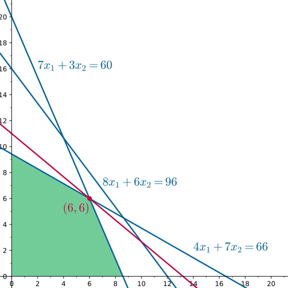
We next maximize $z=5x_1+6x_2$. Treating this equation as the line $5x_1+6x_2=z$, varying $z$ gives a family of parallel lines; larger $z$ moves the line farther toward the upper right. Move the line until it reaches a critical position where any further movement makes it miss the depicted region. The corresponding $z$ is the maximum.

As shown, this occurs at the red point, the intersection of $4x_1 + 7x_2 = 66$ and $7x_1 + 3x_2 = 60$. Solving the two equations gives $(6,6)$. This is the unique optimum, and the cook's maximum profit is $z=66$.

When there are more than two decision variables, the graphical method no longer applies. Some observations from this example remain valid: each inequality constraint describes a half-plane, and the feasible set is their intersection, hence a convex polygon. An optimum can always be attained at a vertex of this polygon, whose coordinates can be found by solving equations for the boundaries of the half-planes. Extending these observations to higher dimensions leads to the simplex method, an efficient method for solving linear programs and the one most often used in programming contests.

Another point is that, in principle, the numbers of buns and dough sticks are integers rather than infinitely divisible quantities. The problem does not explicitly impose this, but its optimum happens to be integral, so adding integrality does not change the answer. In many programs, however, an optimum need not occur at an integer point; such problems are integer programs rather than ordinary linear programs. This class is briefly discussed at the end.

Basic Concepts

This section introduces basic concepts of linear programming.

Linear Programs

A linear program $P$ usually consists of two parts:

• A linear objective function of the form

  $$f(x_1,x_2,\cdots,x_n)=c_1x_1+c_2x_2+\cdots+c_nx_n$$

  where $c_i\in\mathbf R$ are constants;

• Linear constraints of the form

  $$g_j(x_1,x_2,\cdots,x_n)=a_{j1}x_1+a_{j2}x_2+\cdots+a_{jn}x_n \le (=,\ge) b_j$$

  where $a_{ji},b_j\in\mathbf R$ are constants.

A linear program maximizes or minimizes its objective subject to the given constraints. A solution $(x_1,x_2,\cdots,x_n)\in\mathbf R^n$ satisfying the constraints is a feasible solution; among feasible solutions, one attaining the optimum objective value is an optimal solution.

Standard Form

For convenient description and further processing, we choose a standard form for linear programs. Different references use different conventions; here the standard form is:

$$\begin{aligned} \min_{\{x_i\}}\;& \sum_{i=1}^n c_ix_i \\ \text{subject to }& \sum_{i=1}^n a_{ji}x_i = b_i \ge 0,~j=1,\cdots,m,\\ & x_i \ge 0,~i = 1,\cdots,n. \end{aligned}$$

In other words, this is a minimization problem in which all decision variables are nonnegative and the only other constraints are equalities with nonnegative right-hand sides. Using matrices gives a more concise expression:

$$\max\{c^Tx : Ax = b \ge 0,~ x\ge 0\}.$$

Here $x=(x_i)\in\mathbf R^n$ is the decision vector, while $b=(b_j)\in\mathbf R^m$ and $A=(a_{ji})\in\mathbf R^{m\times n}$ are constants in the constraints. The size of a linear program means the number of decision variables and constraints.

Vector Inequalities

Vector inequalities such as $b \ge 0$ occur repeatedly in this article. In general, for vectors $x,y\in\mathbf R^n$, the inequality $x\le y$ means $\forall i(x_i\le y_i)$, comparing real values coordinate by coordinate. This relation is a partial order on the vector space, so some pairs of vectors are incomparable.

The choice of standard form is only for convenience. It is not special, because every linear program can equivalently be written in one of the following six forms:

$$\begin{aligned} &\min\{c^Tx : Ax = b,~ x\ge 0\},\\ &\min\{c^Tx : Ax \ge b\},\\ &\min\{c^Tx : Ax \ge b,~ x\ge 0\},\\ &\max\{c^Tx : Ax = b,~ x\ge 0\}, \\ &\max\{c^Tx : Ax \le b\},\\ &\max\{c^Tx : Ax \le b,~ x\ge 0\}.\\ \end{aligned}$$

The following operations convert any linear program equivalently into one of these six forms:

1. Multiplying by a negative sign, replacing $c$ with $-c$, converts maximization to minimization and vice versa.
2. Multiplying by a negative sign, replacing $a_j^Tx \lesseqqgtr b_j$ with $-a_j^Tx \gtreqqless -b_j$, reverses an inequality or makes the right-hand side of an equality nonnegative.
3. Every equality $a_j^Tx = b_j$ can be replaced by the two opposite inequalities $a_j^Tx \ge b_j$ and $a_j^Tx \le b_j$.
4. Every inequality $a_j^Tx \le(\ge) b_j$ can be converted by adding a nonnegative slack variable $s_j$ into the equality $a_j^Tx +(-) s_j = b_j$ together with $s_j\ge 0$.
5. If a decision variable $x_i$ is unrestricted in sign, replace it by the difference of two nonnegative variables: $x_j = x^+_j - x^-_j$ with $x^+_j,x^-_j \ge 0$.

The transformed program has size at most twice that of the original, and feasible and optimal solutions can be converted easily in both directions. Thus a general linear program can first be converted to standard form (or one of the six forms) before being solved.

Example

Consider the linear program

$$\begin{aligned} \max\;& 3x_1 - 2x_2 + x_3 \\ \text{subject to }& 2x_1 + 3x_2 + 4x_3 \ge 1,\\ & 3x_1 + 4x_2 \le 5,\\ & 5x_2 - x_3 = -1, \\ & x_1, x_2 \ge 0. \end{aligned}$$

Operations 1, 2, and 3 convert it into the form $\min\{c^Tx : Ax \ge b\}$, namely

$$\begin{aligned} \min\;& -3x_1 + 2x_2 - x_3 \\ \text{subject to }& 2x_1 + 3x_2 + 4x_3 \ge 1,\\ & -3x_1 - 4x_2 \ge -5,\\ & 5x_2 - x_3 \ge -1, \\ & -5x_2 + x_3 \ge 1, \\ & x_1 \ge 0,\\ & x_2 \ge 0. \end{aligned}$$

Operations 4 and 5 convert it into the form $\max\{c^Tx : Ax = b,~ x\ge 0\}$, namely

$$\begin{aligned} \max\;& 3x_1 - 2x_2 + x^+_3 - x^-_3 \\ \text{subject to }& 2x_1 + 3x_2 + 4x^+_3 - 4x^-_3 - x_4 = 1,\\ & 3x_1 + 4x_2 + x_5 = 5,\\ & 5x_2 - x^+_3 + x^-_3 = -1, \\ & x_1, x_2, x^+_3, x^-_3, x_4, x_5 \ge 0. \end{aligned}$$

Feasible Regions and Solutions

The set of all feasible solutions $\mathcal D\subseteq\mathbf R^n$ is the feasible region of $P$. Geometrically, each inequality $a_j^T x \le b_j$ describes a half-space $\{x\in\mathbf R^n:a_j^T x \le b_j\}$, and each equality $a^T_jx = b_j$ describes a hyperplane $\{x\in\mathbf R^n:a_j^Tx=b_j\}$. Thus the feasible region is an intersection of finitely many half-spaces and hyperplanes. In optimization¹，such a geometric object is called a polyhedron in $\mathbf R^n$. A polyhedron is always closed and convex but need not be bounded. A bounded polyhedron is also called a polytope. A polytope generalizes a polygon to higher dimensions, while a polyhedron further allows unboundedness.

Examples of Polyhedra

Here are some common polyhedra:

1. The empty set $\varnothing$, also called a nullitope, with dimension defined as $-1$.
2. An affine subspace, the intersection of several hyperplanes $\{x\in\mathbf R^n:Ax = b\}$. It is the solution set of the linear system $Ax = b$: if the system is inconsistent, it is empty; otherwise, it can always be written as $x_0+V$, where $x_0\in\mathbf R^n$ and $V\subseteq\mathbf R^n$ is an $n-\operatorname{rank}(A)$-dimensional linear subspace. In particular, a hyperplane is also an affine subspace.
3. A polyhedral cone, the set of all nonnegative combinations of finitely many points $\{x_i\}$, namely $\{\sum_i\alpha_ix_i:\alpha_i\ge 0\}$. It is a convex cone with its apex at the origin. Equivalently, it is the polyhedron bounded by hyperplanes through the origin, $\{x\in\mathbf R^n : Ax\le 0\}$. In particular, a half-space is also a polyhedral cone.
4. A polytope, namely a bounded polyhedron. In particular, the $-1$-, $0$-, $1$-, $2$-, and $3$-dimensional polytopes are the familiar empty set, point, segment, polygon, and (in the usual sense) polyhedron. A set is a polytope if and only if it is the convex hull of finitely many points $\{x_i\}$, namely $\{\sum_i\alpha_ix_i:\alpha_i\ge 0,~\sum_i\alpha_i=1\}$. A $k$-dimensional polytope is generated by at least $k+1$ points.
5. A simplex, namely a polytope generated by exactly $k+1$ points and of dimension $k$. It is the simplest $k$-dimensional polytope. In particular, the $-1$-, $0$-, $1$-, $2$-, and $3$-dimensional polytopes are the empty set, point, segment, triangle, and tetrahedron. The simplest $k$-dimensional simplex is $\{x\in\mathbf R^k:x_i\ge 0,~\sum_ix_i=1\}$, and every $k$-dimensional simplex can be transformed into this special case by an affine transformation (translation and scaling). Note that the simplex method is not actually performed on a simplex.

Every polyhedron can be viewed as the Minkowski sum: the former describes the unbounded part and the latter the shape of the bounded part. This polyhedral cone is unique: the polyhedral cone in the decomposition of $\{x\in\mathbf R^n:Ax\le b\}$ is always $\{x\in\mathcal R^n:Ax\le 0\}$.

Solutions of linear programs are closely related to polyhedral structure. For a polyhedron $\mathcal D\in\mathbf R^n$ and a vector $c\in\mathbf R^n\setminus\{0\}$, consider the program $P$ below (the minimization case is analogous):

$$\max\{c^Tx:x\in\mathcal D\}.$$

Geometrically, given the hyperplane $H:c^Tx = z$ and the feasible region $\mathcal{D}$, move in the direction of $c$ the hyperplane $H$ while keeping it intersecting the region, and make $z$ as large as possible. There are three possibilities:

• The feasible region $\mathcal D$ is empty. Then $P$ has no feasible solution because some constraints contradict one another. $P$ is infeasible, and its optimum is defined as $-\infty$.

• The feasible region $\mathcal D$ is nonempty but contains a ray in direction $c$: some $x_0\in\mathbf R^n$ satisfies $x_0+tc\in\mathcal D$ for every $t\ge 0$. Because along direction $c$ the hyperplane $H$ can keep moving, and $H\cap\mathcal D$ remains nonempty, the objective $c^Tx = c^Tx_0 + tc^Tc$ can be arbitrarily large. Then $P$ is unbounded, and its optimum is defined as $+\infty$.

• The feasible region $\mathcal D$ is nonempty and contains no ray in direction $c$. Then problem $P$ is bounded. Let $z^*\in\mathbf R$ be the optimum of problem $P$. The hyperplane $H^*:c^Tx = z^*$ is critical: it intersects the polyhedron $\mathcal D$, and $\mathcal D$ lies in the half-space $\{x:c^Tx\le z^*\}$. This hyperplane is a supporting hyperplane of the polyhedron $\mathcal D$. The optimal set of $P$ is $H^*\cap\mathcal D$. As the intersection of a supporting hyperplane and a polyhedron, $H^*\cap\mathcal D$ is a polyhedron contained in the boundary of $\mathcal D$. It is called a face of $\mathcal D$. Informally, the polyhedron is bounded by these faces. In addition to faces formed this way, a polyhedron generally has two more faces: the empty set and the polyhedron itself. Ordered by inclusion, all faces form a lattice structure.

  A face of a $d$-dimensional polyhedron has an integer dimension between $0$ and $d$. A $0$-dimensional face (a point) is a vertex or corner point of polyhedron $\mathcal D$; a $1$-dimensional face is an edge of $\mathcal D$; and a $d-1$-dimensional face is a facet of $\mathcal D$. Not every polyhedron has vertices. Since a face of a face is still a face, and only affine subspaces have no strictly smaller nonempty face, all minimal faces of $\mathcal D$ are affine subspaces. The minimal faces of the same polyhedron have the same dimension; in particular, the minimal faces of $\mathcal D=\{x\in\mathbf R^n:Ax\le b\}$ have dimension $n-\operatorname{rank}A$.

  A face of a polyhedron is the solution set of a bounded linear program, so we need to determine the equations of its faces. Suppose the polyhedron is described by constraints $\mathcal D$, and $a_j^Tx \lesseqqgtr b_j$ is a face of $F$. If a constraint is an equality for every $\mathcal D$, it is tight on $x\in F$. Points of $F$ satisfy the equations obtained from these tight constraints, and the intersection of the resulting affine subspace with $F$ is $\mathcal D$. Conversely, choosing any subset of the constraints of $F$, setting them to equality, and intersecting the resulting affine subspace with $\mathcal D$ gives a face of $\mathcal D$. The more tight constraints are chosen, the smaller the face under inclusion.

  In particular, the feasible region $\mathcal D=\{x\in\mathbf R^n:Ax=b,~x\ge 0\}$ of standard form has coefficient matrix $\begin{pmatrix}A\\ I\end{pmatrix}$ of rank $n$, so its minimal faces are vertices. Thus, if the problem is bounded, an optimum can be chosen at a vertex, obtained by solving $n$ linearly independent tight constraints. This is a convenience of standard form.

Example

In the figure, $\mathcal D$ is the feasible region. Objective coefficients $c_1,c_2,c_3$ give, respectively, a unique optimum, multiple optima, and an unbounded problem. In the first two cases, the corresponding thick red line is a supporting hyperplane of $\mathcal D$; the optimal sets are the vertex $B$ and edge $\overline{CD}$. In the third case, $\mathcal D$ contains a ray in direction $c_3$, so a hyperplane with normal $c_3$ can keep moving in the direction of $c_3$, and the problem is unbounded.

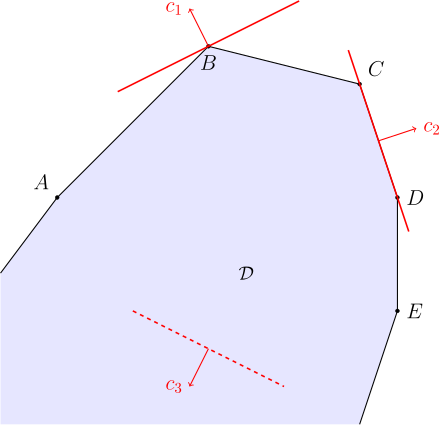
The discussion above ignores $c=0$. Then the program cannot be unbounded: it is either infeasible, or its optimum is $0$ and its optimal set is all of $\mathcal D$. This special type is called feasibility linear programming.

It is worth noting that deciding feasibility or boundedness of a linear program, and finding a feasible solution to a system of inequalities, are just as difficult as solving the linear program itself². For example, the proof of the strong duality theorem below shows that solving a bounded linear program is equivalent to finding a feasible solution to a system of inequalities. Therefore, for tasks such as deciding whether a system of inequalities has a solution or whether a system of equations has a nonnegative solution, the most effective approach is to solve the corresponding feasibility linear program³.

If a constraint is tight on no face of the feasible region, it is redundant. In the cook's example at the beginning, the time constraint is redundant. To determine whether $a_j^Tx\le b_j$ is redundant in a system, solve $\max\{a_j^Tx:x\in\mathcal D\}$ and compare it with $b_j$.

Common Algorithms

In programming contests, few problems can only be solved by a linear-programming algorithm. Most problems solvable by linear programming can usually be solved more efficiently by specialized algorithms such as network flow.

Common algorithms for linear programming are:

• Simplex method
• Ellipsoid method
• Interior-point method

Although the simplex method has exponential worst-case complexity and interior-point methods have polynomial complexity, both perform extremely well in most practical problems. The ellipsoid method also has polynomial theoretical complexity, but is usually slow and impractical.

It is not currently known whether linear programming has a strongly polynomial-time algorithm.

Dual Problems

Every linear program has a corresponding dual problem. Their solutions are closely related. The dual can reveal the structure of the original problem and often improve the efficiency of solving it.

For the linear program $P$ (lowercase variables here are vectors)

$$\begin{aligned} \min_{x_1,x_2,x_3}\;& c_1^Tx_1 + c_2^Tx_2 + c_3^Tx_3 \\ \text{subject to }& A_{11}x_1 + A_{12}x_2 + A_{13}x_3 \ge b_1,\\ & A_{21}x_1 + A_{22}x_2 + A_{23}x_3 = b_2,\\ & A_{31}x_1 + A_{32}x_2 + A_{33}x_3 \le b_3,\\ & x_1\ge 0,~ x_3\le 0, \end{aligned}$$

its dual problem $D$ is the linear program

$$\begin{aligned} \max_{y_1,y_2,y_3}\;&b_1^Ty_1+b_2^Ty_2+b_3^Ty_3 \\ \text{subject to }&A_{11}^Ty_1 + A_{21}^Ty_2 + A_{31}^Ty_3\le c_1,\\ &A_{12}^Ty_1 + A_{22}^Ty_2 + A_{32}^Ty_3 = c_2,\\ &A_{13}^Ty_1 + A_{23}^Ty_2 + A_{33}^Ty_3 \ge c_3,\\ &y_1\ge 0,~ y_3\le 0. \end{aligned}$$

The dual variables $y_1,y_2,y_3$ are the Lagrange multipliers for the three types of constraints in the original problem. Conversely, $x_1,x_2,x_3$ are the Lagrange multipliers for the three types of constraints in the dual. It is easy to verify that the dual of the dual is the original problem.

The correspondence between $P$ and $D$ is:

In particular, the dual of the standard-form program

$$\min\{c^Tx:Ax=b,~x\ge 0\}$$

is

$$\max\{b^Ty:A^Ty\le c\}.$$

Duality Principle

The original and dual problems are not only mirror images in form; their solutions are also closely related. This is the duality principle. For convenience, the theorems and proofs below use the standard-form primal problem.

First, the weak duality theorem says that the maximum of the dual is no greater than the minimum of the primal.

Weak duality theorem

For every $A\in\mathbf R^{m\times n}$, $b\in\mathbf R^m$, and $c\in\mathbf R^n$, we have

$$\max\{b^Ty:A^Ty\le c\} \le \min\{c^Tx:Ax=b,~x\ge 0\}.$$

Proof

If either the primal or dual is infeasible, the inequality is trivial. Assume both are feasible. For every feasible $x$ and $y$,

$$b^Ty = x^TA^Ty \le x^Tc.$$

Taking the extrema on both sides proves weak duality.

Weak duality leaves only four possible situations for the primal and dual:

1. Both are infeasible, namely $-\infty\le+\infty$；
2. The primal is infeasible and the dual is unbounded, namely $+\infty\le+\infty$；
3. The primal is unbounded and the dual is infeasible, namely $-\infty\le-\infty$；
4. Both are bounded.

Weak duality has many corollaries. For example, it gives a way to detect primal unboundedness from primal and dual feasibility.

Corollary

A linear program is unbounded if and only if it is feasible and its dual is infeasible.

Applying weak duality to feasibility linear programs gives Farkas' lemma and its variants.

Farkas' lemma

For $A\in\mathbf R^{m\times n}$ and $b\in\mathbf R^n$, exactly one of the following holds:

1. There is an $x\in\mathbf R^n$ with $Ax=b$ and $x\ge 0$;
2. There is a $y\in\mathbf R^m$ with $A^T y\ge 0$ and $b^Ty<0$.

Proof

Consider $\max\{0:Ax=b,~x\ge 0\}$, whose dual is $\min\{b^Ty:A^Ty\ge 0\}$. The dual is feasible because $0\in\mathbf R^m$ is feasible. By weak duality, either the primal is feasible or the dual is unbounded, but not both. These are exactly cases 1 and 2 of Farkas' lemma.

Farkas' lemma is in fact a hyperplane separation theorem. Case 1 says that the point $b$ lies in the polyhedral cone generated by the columns of $A$, $C$; therefore, Farkas' lemma says that, if and only if the point $b$ is not in this convex cone $C$, there is a hyperplane with normal vector $y$, $H:y^Tx = 0$, through the origin that strictly separates the point $b$ from the cone $C$.

In the fourth case allowed by weak duality, a stronger conclusion holds: the primal and dual optima are equal. Combining this with the other three cases gives strong duality: whenever either the primal or the dual is feasible, their optimal values are equal.

Strong duality theorem

For every $A\in\mathbf R^{m\times n}$, $b\in\mathbf R^m$, and $c\in\mathbf R^n$,

$$\max\{b^Ty:A^Ty\le c\} = \min\{c^Tx:Ax=b,~x\ge 0\}.$$

provided at least one of the two sets is nonempty.

Proof

The only case not covered by weak duality is when both primal and dual are feasible. Consider the following feasibility program $Q$:

$$\max\{0:c^Tx \le b^Ty,~Ax=b,~x\ge 0,~A^Ty\le c\}.$$

If $Q$ has a feasible solution $(x^*,y^*)\in\mathbf R^n\times\mathbf R^m$, weak duality and optimality give

$$b^Ty^* \le \max\{b^Ty:A^Ty\le c\} \le \min\{c^Tx:Ax=b,~x\ge 0\} \le c^Tx^*,$$

But $c^Tx^*\le b^Ty^*$, so all inequalities are equalities. Thus strong duality holds, and $x^*$ and $y^*$ are optimal primal and dual solutions.

It remains to prove that $Q$ is feasible. Suppose not. As in the proof of Farkas' lemma, consider problem $Q$'s dual $DQ$:

$$\min\{c^T\mu - b^T\lambda : ct - A^T\lambda \ge 0,~ -bt + A\mu = 0,~t\ge 0,~\mu\ge 0\}.$$

Since $(t,\lambda,\mu)=(0,0,0)$ is feasible for $DQ$, weak duality says that infeasibility of $Q$ implies unboundedness of $DQ$. Thus some $(t^*,\lambda^*,\mu^*)$ satisfies

$$c^T\mu^* - b^T\lambda^* <0,~ ct^* - A^T\lambda^* \ge 0,~ -bt^* + A\mu^* = 0,~t^*\ge 0,~\mu^*\ge 0.$$

If $t^*>0$, these inequalities make $(x,y)=(\mu^*/t^*,\lambda^*/t^*)$ feasible for the preceding problem, a contradiction. Hence $t^*=0$, so

$$c^T\mu^* < b^T\lambda^*,~ A^T\lambda^*\le 0,~ A\mu^*=0,~\mu^*\ge 0.$$

However, since both the primal and dual in the theorem are assumed feasible, some $(x_0,y_0)$ satisfies

$$Ax_0 = b,~ x_0\ge 0,~ A^Ty_0\le c$$

and therefore

$$0 = (A\mu^*)^Ty_0 = (A^Ty_0)^T\mu^* \le c^T\mu^* < b^T\lambda^* = x_0^TA^T\lambda^* \le 0.$$

This is a contradiction. Hence $Q$ is feasible, and strong duality follows.

The proof of strong duality also gives:

Corollary

If feasible primal and dual solutions $x^*$ and $y^*$ satisfy strong duality, $c^Tx^* = b^Ty^*$, then they are optimal solutions to the primal and dual, respectively.

Strong duality says that for a feasible linear program, solving the dual is enough to obtain the primal optimum.

Complementary Slackness

As in other optimization problems, complementary slackness is part of the optimality conditions. Since the objective is linear, for linear programs it is also necessary and sufficient for feasible solutions to be optimal.

The complementary slackness condition says that a variable in the dual (primal) can be nonzero only when the corresponding constraint in the primal (dual) is an equality, or tight. If a nonzero variable is viewed as a slack constraint, this says that corresponding variables and constraints in the primal and dual cannot both be slack.

For a standard-form linear program:

Theorem

Suppose $x^*$ and $y^*$ are feasible solutions to the primal $\min\{c^Tx:Ax=b,~x\ge 0\}$ and dual $\max\{b^Ty:A^Ty\le c\}$ Then they are both optimal if and only if complementary slackness holds, namely

$$x^T(A^Ty-c) = 0$$

then $x^*$ and $y^*$ are optimal solutions to the primal and dual, respectively.

Proof

Since $x^*$ and $y^*$ are feasible,

$$b^Ty^* - c^Tx^* = (x^*)^T(A^T y^* - c).$$

Thus complementary slackness holds if and only if $b^Ty^* = c^Tx^*$. By the strong-duality corollary, this is equivalent to $x^*$ and $y^*$ being optimal.

Standard form may be too restrictive. A slightly more general version is:

Theorem

Suppose $x^*$ and $y^*$ are feasible solutions to the primal $\min\{c^Tx:Ax\ge b,~x\ge 0\}$ and dual $\max\{b^Ty:A^Ty\le c,~y\ge 0\}$ Then they are both optimal if and only if complementary slackness holds, namely

$$x^T(A^Ty-c) = y^T(Ax-b) = 0$$

Then $x^*$ and $y^*$ are optimal solutions to the primal and dual, respectively.

Proof

The proof is essentially the same, except that the difference is written as

$$b^Ty^* - c^Tx^* = (x^*)^T(A^T y^* - c) - (y^*)^T(Ax^*-b).$$

Complementary slackness provides a simple test for optimality of feasible solutions to a linear program.

Primal-Dual Method

The dual can assist in solving the primal. A common approach is the primal-dual method, which solves a sequence of relatively simple auxiliary problems to improve a dual solution and eventually obtain an optimal primal solution.

For the standard-form primal

$$(P)\qquad\min\{c^Tx : Ax=b\ge 0,~ x\ge 0\}$$

and its dual

$$(D)\qquad\max\{b^Ty : A^Ty\le c\},$$

The previous section showed that it suffices to find feasible solutions to $(P)$ and $(D)$ satisfying complementary slackness $x^T(A^Ty-c)=0$. Consider the following procedure:

1. Start from a feasible dual solution to $(D)$, namely $y$, and compute the set of tight dual constraints

   $$I = \{i : (A^Ty - c)_i = 0\}.$$

2. By complementary slackness, if there is a feasible solution to $(P)$, denoted $x$, with $x_i>0$ only when $i\in I$, we have found optimal solutions. Thus consider the linear program

   $$(RP)\qquad \begin{aligned} \min_{x,s}\;& \mathbf 1^Ts \\ \text{subject to } & Ax + s = b, \\ & x_i \ge 0,~\forall i \in I,\\ & x_i = 0,~\forall i \notin I,\\ & s \ge 0. \end{aligned}$$

3. If the minimum of $(RP)$ is $0$, then the optimum $(x^*,0)$ has $x^*$ as an optimum of the primal $(P)$. Otherwise, solve the dual $(DRP)$ for $\bar y$:

   $$(DRP)\qquad \begin{aligned} \max_{y}\;& b^Ty \\ \text{subject to }& \sum_{j}a_{ji}y_j \le 0,~\forall i\in I,\\ & y \le 1. \end{aligned}$$

   Strong duality gives $b^T\bar y = 1^Ts^*>0$.

4. Use the solution of $(DRP)$ to improve the feasible solution of $(D)$. Let $y' = y + \varepsilon \bar y$ with $\varepsilon>0$. Then $b^Ty' = b^Ty + \varepsilon b^T\bar y > b^Ty$. Choose $y'$ as large as possible while keeping $(D)$ feasible for $\varepsilon$.

   For $i\in I$,

   $$\sum_ja_{ji}y'_j = \sum_ja_{ji}y_j + \varepsilon \sum_ja_{ji}\bar y_j \le c_i,$$

   so these constraints of $(D)$ remain satisfied.

   For the remaining constraints, $i\notin I$, take

   $$\varepsilon = \min\left\{\dfrac{c_i - \sum_{j}a_{ji}y_j}{\sum_{j}a_{ji}\bar y_j}:i\notin I,~\textstyle\sum_{j}a_{ji}\bar y_j>0\right\}$$

   This improves the dual as much as possible while preserving feasibility; then return to step 1. If the set in the formula is empty, so $\varepsilon=+\infty$, the dual $(D)$ is unbounded and the primal $(P)$ is infeasible.

Only $(DRP)$ truly needs to be solved; strong duality links problem $(RP)$ to $(DRP)$. Problem $(D)$ supplies a direction for improving the dual solution and has a simpler form than the dual $(DRP)$. Farkas' lemma guarantees feasibility of problem $(DRP)$, while the constraint $y\le 1$ is a normalization condition that makes problem $(DRP)$ bounded.

In programming contests, the primal-dual method is widely used in combinatorial optimization. Examples include the Hungarian algorithm, the cycle-canceling algorithm for minimum-cost flow, the SSP algorithm (primal-dual algorithm), Dijkstra's algorithm for shortest paths, and the Ford–Fulkerson augmenting algorithm for maximum flow; all can be viewed as direct applications of the primal-dual method.

Integer Programming

Integer programming usually means integer linear programming (ILP). Its standard form is:

$$\begin{aligned} \min_{x}\; & c^Tx \\ \text{subject to } & Ax = b \ge 0,\\ & x \ge 0,\\ & x \in \mathbf Z^n, \end{aligned}$$

Here $A\in\mathbf R^{m\times n}$, $b\in\mathbf R^m$, and $c\in\mathbf R^n$. An ILP is obtained by adding the requirement that the decision variables of a linear program be integers.

Integer constraints substantially increase complexity. Many combinatorial optimization problems, such as knapsack, satisfiability, and numerous graph-optimization problems, can be modeled as ILPs, and most of them are known to be NP-hard.

Totally Unimodular Matrices

For this reason, large integer optimization problems are sometimes relaxed by dropping integrality and solving an LP instead. For minimization, the relaxed LP optimum is generally only a lower bound for the ILP optimum. If the relaxed optimum happens to be integral, it is also an optimum of the original ILP.

A natural question is whether some condition guarantees that every LP optimum is integral. Totally unimodular matrices provide such a condition.

Totally unimodular matrix

A matrix $A\in\mathbf R^{m\times n}$ is totally unimodular if every square submatrix has determinant $0$ or $\pm 1$. The matrix $A$ is therefore called totally unimodular.

In particular, every entry of a totally unimodular matrix is $0$ or $\pm 1$. This gives the following result:

Theorem

For a totally unimodular matrix $A\in\mathbf Z^{m\times n}$, $b\in\mathbf Z^{m}$, and $c\in\mathbf Z^n$, the LP and its dual

$$\min\{c^Tx : Ax=b,x\ge 0\} = \max\{b^Ty: A^Ty\le c\}$$

have integer optima whenever they are bounded.

Proof

Earlier we saw that an LP optimum can be chosen on a minimal face, which is the solution set of the equations from several linearly independent tight constraints:

$$\{x\in\mathbf R^n : a_j^Tx = b_j,~\forall j\in J\}.$$

Write this system as $A_Jx=b_J$, with $A_J=(A_1,A_2)$, where $A_1$ is a full-rank square matrix with determinant $\pm 1$. By Cramer's rule, the solution

$$x = \begin{pmatrix}A_1^{-1}b_J \\ 0\end{pmatrix}$$

is an integer solution on the minimal face.

In common graph models, the coefficient matrices of the LPs for network flow, shortest path, and bipartite graphs are totally unimodular. If the parameters are integral, their optima can therefore be chosen integral, with no fractional flows or matchings. Thus maximum flow, minimum cut, minimum-cost flow, shortest path, difference constraints, and maximum (weight) matching and minimum vertex cover in bipartite graphs can all be formulated as linear programs. Moreover, maximum flow and minimum cut, shortest path and difference constraints, and maximum bipartite matching and minimum vertex cover are pairwise dual problems.

Some other graph models have feasible solutions exactly equal to all vertices of a polytope whose vertices are integral. By choosing constraints carefully, the corresponding combinatorial optimum is an LP optimum. General-graph matching and spanning-tree models are examples, so general-graph maximum (weight) matching and minimum spanning tree can likewise be formulated as linear programs.

References and Notes

• Schrijver, Alexander. Theory of linear and integer programming. John Wiley & Sons, 1998.
• Papadimitriou, Christos H., and Kenneth Steiglitz. Combinatorial optimization: algorithms and complexity. Courier Corporation, 1998.
• Duality in linear programming. Part 1—definition and construction. by adamant - Codeforces blog
• Duality in linear programming. Part 2—in competitive programming. by adamant - Codeforces blog

Footnotes

1. Different references define these terms differently: some call the bounded case a “polyhedron” and the unbounded case a “polytope”; some do not assume convexity; and some use “polyhedron” for a three-dimensional polytope. This article follows the definitions in Schrijver (1998), Boyd and Vandenberghe (2004), and similar references. ↩

2. More precisely, they are mutually reducible in polynomial time. ↩

3. Other methods for systems of inequalities include Fourier–Motzkin elimination and the Agmon–Motzkin–Schoenberg relaxation method. They are more direct but often inefficient. ↩