Recalling the concept of basis vectors from high-school solid geometry, we can find a set of basis vectors , , and in three-dimensional Euclidean space, after which any vector in the space can be represented by these basis vectors. In other words, we can describe an infinite three-dimensional space using finitely many basis vectors, which is enough to demonstrate the importance of basis vectors.
Three-dimensional Euclidean space is a special linear space, and its basis vectors are generalized to linear bases in linear spaces.
Applications of linear bases in OI usually involve only two kinds of linear spaces: the -dimensional real linear space and the -dimensional linear space over the Boolean domain. We will introduce them in detail in the Applications section. If you are unfamiliar with linear algebra, we recommend starting with the Applications section.
The following discussion introduces linear bases from the perspective of general linear spaces and gives their common properties.
Prerequisite: Linear spaces.
A linear basis is a basis of a linear space and an important tool for studying linear spaces.
Definition
An inclusion-maximal linearly independent set in a linear space is called a Hamel basis or linear basis of , abbreviated as a basis.
The basis of the linear space is defined to be the empty set.
It can be proved that every linear space has a linear basis1. We define the dimension of a linear space as the number of elements (or the cardinality) of a linear basis, denoted by .
Properties
-
For a finite-dimensional linear space of dimension :
-
In , any collection of vectors is linearly dependent.
-
In , any linearly independent vectors form a basis of .
-
If every vector in can be expressed linearly by the vector group , then it is a basis of .
???+ note "Proof" In , take any basis . By the given condition, the vector group can be expressed linearly by , so
$$ n=\operatorname{rank}\{b_1,b_2,\dots,b_n\}\leq\operatorname{rank}\{a_1,a_2,\dots,a_n\}\leq n $$ Therefore, $\operatorname{rank}\{a_1,a_2,\dots,a_n\}=n$. -
In , any linearly independent vector group can be made into a basis of by inserting some vectors.
-
-
(The subspace dimension formula.) Let be finite-dimensional linear spaces over , and suppose that and are also finite-dimensional. Then .
???+ note "Proof" Let , , and .
Take a basis of $V_1\cap V_2$, denoted by $a_1,a_2,\dots,a_m$, and extend it to bases of $V_1$ and $V_2$, respectively: $a_1,a_2,\dots,a_m,b_1,b_2,\dots,b_{n_1-m}$ and $a_1,a_2,\dots,a_m,c_1,c_2,\dots,c_{n_2-m}$. It remains only to prove that the vector group $a_1,a_2,\dots,a_m,b_1,b_2,\dots,b_{n_1-m},c_1,c_2,\dots,c_{n_2-m}$ is linearly independent. Let $\sum_{i=1}^m r_ia_i+\sum_{i=1}^{n_1-m} s_ib_i+\sum_{i=1}^{n_2-m} t_ic_i=\theta$. Then $\sum_{i=1}^{n_2-m} t_ic_i=-\sum_{i=1}^m r_ia_i-\sum_{i=1}^{n_1-m} s_ib_i$. The left side lies in $V_2$ and the right side lies in $V_1$, so both sides lie in $V_1\cap V_2$. Therefore, $\sum_{i=1}^{n_2-m} t_ic_i=\sum_{i=1}^m k_ia_i$. Hence $t_1=t_2=\dots=t_{n_2-m}=k_1=k_2=\dots=k_m=0$, and consequently $r_1=r_2=\dots=r_m=s_1=s_2=\dots=s_{n_1-m}=t_1=t_2=\dots=t_{n_2-m}=0$. -
Let be finite-dimensional linear spaces over , and suppose that and are also finite-dimensional. The following statements are equivalent:
-
.
-
.
-
If is a basis of and is a basis of , then is a basis of .
???+ note "Note" Statements 1 and 3 can be generalized to infinite-dimensional linear spaces.
-
Examples
Consider bases of .
-
As shown in the figure:
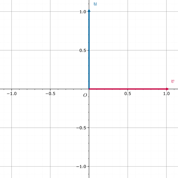
form a basis.
-
As shown in the figure:
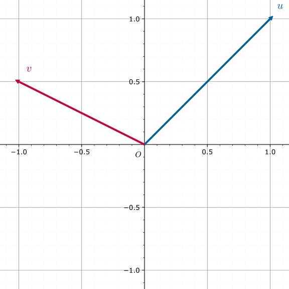
form a basis.
-
As shown in the figure:
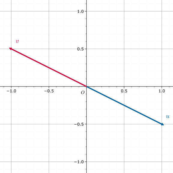
do not form a basis because .
-
As shown in the figure:
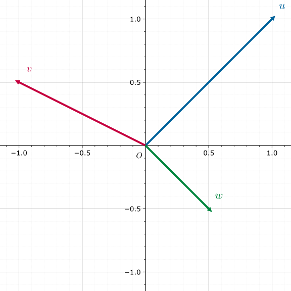
do not form a basis because .
Orthogonal Bases and Orthonormal Bases
If a linear space has a basis satisfying (that is, its elements are pairwise orthogonal), then this basis is called an orthogonal basis.
If a linear space has an orthogonal basis that also satisfies , this basis is called an orthonormal basis.
The basis of any finite-dimensional linear space can be transformed into an orthogonal basis through Schmidt orthogonalization.
Applications
Based on the preceding discussion, linear bases can be used to:
- Find the rank of a given vector group;
- Find a maximal linearly independent set (or a basis of its span) for a given vector group;
- Insert some vectors into a given vector group and find a maximal linearly independent set (or a basis of its span) in the resulting vector group;
- Determine whether a vector can be expressed linearly by a maximal linearly independent set (or basis) that has been found;
- Find special elements in the span of a maximal linearly independent set (or basis) that has been found, such as the maximum or minimum element.
In OI, a linear basis of the -dimensional real linear space is generally called a real linear basis, while a linear basis of the -dimensional Boolean-domain linear space is called an XOR linear basis.
Tip
Addition in is XOR and multiplication is AND; one can prove that is a field.
One can prove that the algebraic system is a linear space, where:
That is, addition is XOR and scalar multiplication is AND.
Taking an XOR linear basis as an example, for a given set of Boolean sequences , we can construct an XOR linear basis with the following properties:
- The XOR sum of any nonempty subset of is not ;
- For , any element can be obtained by taking some elements from whose XOR sum is ;
- For any set satisfying the preceding two conditions, the number of its elements is no smaller than the number of elements in .
An XOR linear basis can be used to:
- Determine whether a number can be represented as the XOR sum of a subset of a given set of numbers;
- Count the ways to represent a number as the XOR sum of a subset of a given set of numbers;
- Find the maximum, minimum, -th largest, or -th smallest XOR sum of a subset of a given set of numbers;
- Find the rank of a number among the XOR sums of subsets of a given set of numbers.
Construction
Since XOR linear bases and real linear bases have no essential difference, we use XOR linear bases as the example below; the code for a real linear basis only requires minor modifications.
Greedy Method
Convert each number in the original set to binary and scan from the highest bit to the lowest. If bit is and does not exist, set and end the scan; if it exists, set .
To query the maximum value of over any number of elements from the original set, scan the linear basis from the highest bit to the lowest. If applying the current operation to makes the answer larger, XOR the answer with .
Why does this work? When scanning from high to low bits, if we have reached bit , we can ensure that bit of the answer is , and no later operation can change bit .
The minimum value of over any number of elements from the original set is simply the smallest element in the linear-basis set.
To query whether a number can be obtained by XOR, proceed similarly to insertion: if the number left at the end of insertion has been XORed to , it can be obtained.
Code (Luogu P3812 [Template] Linear Basis)
#include <algorithm>
#include <iostream>
using ull = unsigned long long;

ull p[64];

void insert(ull x) {
  for (int i = 63; ~i; --i) {
    if (!(x >> i))  // Bit i of x is 0
      continue;
    if (!p[i]) {
      p[i] = x;
      break;
    }
    x ^= p[i];
  }
}

using std::cin;
using std::cout;

int main() {
  int n;
  cin >> n;
  ull a;
  for (int i = 1; i <= n; ++i) {
    cin >> a;
    insert(a);
  }
  ull ans = 0;
  for (int i = 63; ~i; --i) {
    ans = std::max(ans, ans ^ p[i]);
  }
  cout << ans << '\n';
  return 0;
}
Gaussian Elimination
Gaussian elimination constructs a linear basis from the perspective of a system of linear equations; its correctness is clear.
Code (Luogu P3812 [Template] Linear Basis)
#include <iostream>
using ull = unsigned long long;
constexpr int MAXN = 1e5 + 5;

ull deg(ull num, int deg) { return num & (1ull << deg); }

ull a[MAXN];
using std::cin;
using std::cout;

int main() {
  cin.tie(nullptr)->sync_with_stdio(false);
  int n;
  cin >> n;
  for (int i = 1; i <= n; ++i) cin >> a[i];
  int row = 1;
  for (int col = 63; ~col && row <= n; --col) {
    for (int i = row; i <= n; ++i) {
      if (deg(a[i], col)) {
        std::swap(a[row], a[i]);
        break;
      }
    }
    if (!deg(a[row], col)) continue;
    for (int i = 1; i <= n; ++i) {
      if (i == row) continue;
      if (deg(a[i], col)) {
        a[i] ^= a[row];
      }
    }
    ++row;
  }
  ull ans = 0;
  for (int i = 1; i < row; ++i) {
    ans ^= a[i];
  }
  cout << ans << '\n';
  return 0;
}
Properties
The linear basis constructed by the greedy method has the following properties:
- No subset of the linear basis has XOR sum .
- The highest set bit of each number in the linear basis is different.
The linear basis constructed by Gaussian elimination satisfies the following property:
-
The matrix after Gaussian elimination is a row-reduced echelon matrix.
This property includes the two properties satisfied by the linear basis constructed by the greedy method.
If you do not understand why this property holds, you can read Gaussian elimination.
Here is an example:
5
633 211 169 841 1008
Binary representations:
1001111001
0011010011
0010101001
1101001001
1111110000
Linear basis generated by the greedy method:
1001111001
0100110000
0011010011
0001111010
0000000000
0000010000
0000000000
0000000000
0000000000
0000000000
Linear basis generated by Gaussian elimination:
1000000011
0100100000
0010101001
0001101010
0000010000
0000000000
0000000000
0000000000
0000000000
0000000000
This is a very useful property that makes many problems easier to solve. For example, given some numbers, if we want the maximum XOR of a subset and construct the linear basis greedily, we need to perform another greedy pass: if the current bit of ans is 0, XORing it will improve the answer; if the current bit is 1, it will not. After constructing the basis by Gaussian elimination, we can simply XOR all basis elements and output the result.
For other classic problems, such as querying whether a number can be obtained by XOR or finding the -th largest XOR value, the basis obtained by Gaussian elimination is also more convenient.
Time Complexity
Let the vector length be and the total number of vectors be . The time complexity is . The constant factor of Gaussian elimination is slightly larger.
For a real linear basis, the time complexity is .
Merging Linear Bases
Merging linear bases only requires brute force: insert every vector from one linear basis into the other. The time complexity of one merge is for an XOR linear basis or for a real linear basis.
Intersecting Linear Bases
Strictly speaking, intersecting linear bases means finding a linear basis of the intersection of the two linear spaces that they span. This section presents two algorithms. For both algorithms, the time complexity of one intersection is for an XOR linear basis or for a real linear basis.
Naive Algorithm
Let the two linear bases to be intersected be and . The intersection algorithm only needs the following adjustments to the brute-force linear-basis merge algorithm (using an XOR linear basis as an example):
- Using the linear basis , try to insert its vector into using the greedy method, and initialize the intersection basis as the empty set;
- During insertion, record the contribution of elements from the linear basis to the vector being inserted. Specifically, maintain a new vector , initialized to ; if the vector being inserted is XORed with the vector at position in the linear basis, XOR the contribution with the contribution recorded at position , namely ;
- If insertion succeeds and at position the vector is inserted, set the recorded value at position , namely , to the contribution that produced from elements of , namely ;
- If insertion fails, insert the contribution of the elements of , recorded as , into .
The resulting linear basis is the desired intersection; the algorithm also computes the union of the two linear bases.
Explanation of the Algorithm
Let the merged linear basis be , where is the vector obtained after inserting . Then is also a merged linear basis. Let be the set . The merged basis can then be written as . Moreover, every vector in the sum space has a unique representation of the form
where and . The in this decomposition is the “contribution of elements of the linear basis ” that the preceding algorithm attempts to record. Strictly speaking, it is the contribution of the vectors in that were inserted successfully at the end.
For a successful insertion, the final recorded is the term in this decomposition. Let . Initially, , which is already the correct decomposition of in the basis . When updating to , since , it is enough to update to to preserve the decomposition. Therefore, by induction, when is finally inserted into the merged linear basis, the recorded contribution is the term in the decomposition above.
For an unsuccessful insertion, the vector being inserted will eventually become , and its contribution is then inserted into . Repeating the preceding argument shows that during insertion we still always have , with , but no longer belongs to . This is because, initially, , with . Apart from that, every term XORed into the contribution during updates belongs to . Thus, in fact, .
Why does inserting all the values from unsuccessful insertions into produce a linear basis of the intersection space? First, if insertion of fails, the final result is , where and . Therefore, must lie in the intersection space . Conversely, let be any element of the intersection space. Since , can be represented as a linear combination (XOR sum) of elements of :
where . For each , record the corresponding contribution inserted into as . Then
Note that and both lie in the intersection space, so the left side also lies in the intersection space and can therefore be written as a linear combination of elements of . At the same time, every term on the right either has , or has and . Thus, the right side is a linear combination of elements of . Since is linearly independent, all coefficients are ; that is, . This shows that the contributions of the vectors that could not be inserted together span the intersection space.
According to this explanation, maintaining the contribution during the process is actually maintaining the decomposition ; moreover, when the contribution is finally inserted into , we always have . Thus, whether we maintain the contributions of elements of or of (that is, whether we maintain or ), the result is correct. To maintain the contributions of elements of , only the initialization needs to change: each vector in , denoted , initially has contribution , while an inserted initially has contribution .
The template-problem code is as follows:
Code (Library Checker Intersection of vector spaces)
#include <array>
#include <iostream>

class LinearBasis {
  static constexpr int K = 30;
  std::array<int, K> a;

  // Size of basis.
  int size() const {
    int res = 0;
    for (auto x : a) {
      if (x) {
        ++res;
      }
    }
    return res;
  }

 public:
  LinearBasis() : a{} {}

  // Insert vector x.
  void insert(int x) {
    for (int k = K - 1; ~k && x; --k) {
      if ((x >> k) & 1) {
        if (!a[k]) {
          a[k] = x;
        }
        x ^= a[k];
      }
    }
  }

  // Return a basis for *THIS intersecting RHS.
  LinearBasis intersect(const LinearBasis& rhs) const {
    LinearBasis res;
    std::array<int, K> c = a, b_parts = {};
    for (int i = K - 1; ~i; --i) {
      int x = rhs.a[i], b_part = x;
      for (int k = i; ~k && x; --k) {
        if ((x >> k) & 1) {
          if (!c[k]) {
            c[k] = x;
            b_parts[k] = b_part;
          }
          x ^= c[k];
          b_part ^= b_parts[k];
        }
      }
      res.insert(b_part);
    }
    return res;
  }

  // Output.
  void print() const {
    std::cout << size();
    for (auto x : a) {
      if (x) {
        std::cout << ' ' << x;
      }
    }
    std::cout << '\n';
  }
};

int main() {
  int t;
  std::cin >> t;
  for (; t; --t) {
    LinearBasis a, b;
    int n;
    std::cin >> n;
    for (; n; --n) {
      int x;
      std::cin >> x;
      a.insert(x);
    }
    int m;
    std::cin >> m;
    for (; m; --m) {
      int x;
      std::cin >> x;
      b.insert(x);
    }
    a.intersect(b).print();
  }
  return 0;
}
Zassenhaus Algorithm
Another equivalent approach is the Zassenhaus algorithm, which can also compute the union and intersection of two linear bases simultaneously. Its complexity is exactly the same as above.
The steps are as follows:
- Initialize an empty linear basis of vector length , denoted , whose vectors have the form with both and of length ;
- From , insert each element in the form into ;
- From , insert each element in the form into ;
- In the final linear basis , among all nonzero elements , the components of those with nonzero form a linear basis of the union of and , while, for those with zero , the components form a linear basis of the intersection of and .
The method used to construct the linear basis can be the greedy method or Gaussian elimination, as long as the linear basis in forms a row-echelon matrix.
Comparing the elimination steps in the Zassenhaus algorithm with those in the preceding naive algorithm, it is easy to see that the greedy Zassenhaus algorithm is equivalent to the naive algorithm that maintains the contributions of elements in . If we instead insert all first and then all , the greedy Zassenhaus algorithm is equivalent to the naive algorithm that maintains the contributions of elements in . By the equivalence of the elimination steps, the Zassenhaus algorithm is also correct.
In addition, an independent and more general algebraic proof can be given:
Correctness Proof
Let be a linear space with subspaces and . The algorithm itself amounts to reducing the subspace
to row-echelon form and finding a basis . At the end of the algorithm, the elements of , namely , must be divided into two classes according to whether . Consider the projection map with . Then , and it is easy to verify that
By the relevant theorem on linear maps, .
The first few columns of a row-echelon matrix are still row-echelon matrices. Therefore, the number of rows with is exactly the row rank of , namely ; moreover, the set of their components forms a basis of . There are exactly remaining nonzero rows, all satisfying . For their components, since , we have ; and because are rows of a row-echelon matrix, the vectors are linearly independent. Thus these form a linearly independent set in the intersection space of size , so they must also form a basis of that space.
The template-problem code is as follows:
Code (Library Checker Intersection of vector spaces)
#include <iostream>
#include <vector>

class LinearBasis {
  int K;
  std::vector<long long> a;

 public:
  LinearBasis(int K) : K(K), a(K) {}

  // Insert vector x.
  void insert(long long x) {
    for (int k = K - 1; ~k && x; --k) {
      if ((x >> k) & 1) {
        if (!a[k]) {
          a[k] = x;
        }
        x ^= a[k];
      }
    }
  }

  // Output those not exceeding 2^k.
  void print(int k) const {
    int sz = 0;
    for (int i = 0; i < k; ++i) {
      if (a[i]) {
        ++sz;
      }
    }
    std::cout << sz;
    for (int i = 0; i < k; ++i) {
      if (a[i]) {
        std::cout << ' ' << a[i];
      }
    }
    std::cout << '\n';
  }
};

int main() {
  constexpr int K = 30;
  int t;
  std::cin >> t;
  for (; t; --t) {
    LinearBasis c(K << 1);
    int n;
    std::cin >> n;
    for (; n; --n) {
      int x;
      std::cin >> x;
      c.insert(((long long)x << K) | x);
    }
    int m;
    std::cin >> m;
    for (; m; --m) {
      int x;
      std::cin >> x;
      c.insert((long long)x << K);
    }
    c.print(K);
  }
  return 0;
}
Note that when outputting, we only need to consider vectors whose first bits are all zero.
Extension: Prefix Linear Basis
This section discusses only XOR linear bases and assumes that a single vector can be stored in space and that each individual operation always has complexity.
For repeated queries of the maximum XOR on intervals, a common approach is to combine a cat tree with a linear basis, with time complexity , where is the vector length, is the sequence length, and is the number of queries. Another feasible approach uses a prefix linear basis (also called a timestamp linear basis), reducing the complexity to .
A prefix linear basis maintains, for every prefix of a sequence, the linear bases of all suffixes of that prefix, thereby supporting queries for the linear basis of every interval. Observe that for a prefix , the linear bases of all its suffixes are nested: the linear basis of always contains that of . Thus, there are at most distinct linear bases among these suffixes, and they can always be obtained by gradually adding new vectors to the empty set, from the suffix through all suffixes up to . By this monotonicity, it is enough to mark each added vector with the largest index at which it appears. Then all suffix linear bases can be stored in space. When querying the linear basis of interval , we only need to retain, in the prefix linear basis at , the vectors whose marks satisfy .
For each vector , call its mark its timestamp. A vector in the linear basis can always be represented as the XOR sum of some elements of the original sequence, for example . Among all such possible representations, the maximum of the minimum indices is , namely
This expression merely writes the description in the preceding paragraph in formal language. It suggests that, to maintain the timestamp of each vector in the linear basis, we only need to greedily replace old vectors with the newest possible vectors.
When constructing a linear basis using the greedy method described above, the prefix linear basis makes the following adjustments during construction:
- For every vector retained in the linear basis, store a timestamp , initially setting all of them to ;
- To add the -th vector in the sequence, still scan from the highest bit to the lowest, but also record the current time ;
- If has bit set, compare the timestamp of the existing vector in the linear basis, , with the current time :
- If , that is, the vector being added is newer, set to , update its timestamp to , and continue the insertion using the old XORed with , namely , with the old recorded time ;
- If , that is, the vector being added is older, do not update or ; continue the insertion after XORing with .
In other words, if the current bit can be represented by a newer vector, use the newer vector directly; otherwise retain the original vector. When updating the vector at position , do not store the XOR result at position , because the timestamp of is , which is smaller than the timestamp of the added vector , namely . For the same reason, upward updates during construction by Gaussian elimination may break the timestamp property, so Gaussian elimination is no longer suitable for constructing a prefix linear basis.
The template-problem code is as follows:
Code (Codeforces 1100F Ivan and Burgers)
#include <algorithm>
#include <array>
#include <iostream>
#include <numeric>
#include <vector>

class LinearBasis {
  static constexpr int K = 20;
  std::array<int, K> a, t;

 public:
  LinearBasis() : a{}, t{} {}

  // Insert vector x at time i.
  void insert(int x, int i) {
    for (int k = K - 1; ~k && x; --k) {
      if (((x >> k) & 1)) {
        if (i > t[k]) {
          std::swap(a[k], x);
          std::swap(t[k], i);
        }
        x ^= a[k];
      }
    }
  }

  // Find max xor of subsets of elements from time i till now.
  int query(int i) const {
    int res = 0;
    for (int k = K - 1; ~k; --k) {
      if (t[k] >= i && (res ^ a[k]) > res) {
        res ^= a[k];
      }
    }
    return res;
  }
};

int main() {
  int n;
  std::cin >> n;
  std::vector<int> c(n + 1);
  for (int i = 1; i <= n; ++i) std::cin >> c[i];
  int q;
  std::cin >> q;
  std::vector<std::array<int, 2>> qu(q);
  for (auto& v : qu) std::cin >> v[0] >> v[1];
  std::vector<int> ids(q);
  std::iota(ids.begin(), ids.end(), 0);
  std::sort(ids.begin(), ids.end(),
            [&](int l, int r) -> bool { return qu[l][1] < qu[r][1]; });
  LinearBasis lb;
  std::vector<int> res(q);
  for (int i = 1, j = 0; i <= n; ++i) {
    lb.insert(c[i], i);
    for (; j < q && qu[ids[j]][1] == i; ++j) {
      res[ids[j]] = lb.query(qu[ids[j]][0]);
    }
  }
  for (int x : res) std::cout << x << '\n';
  return 0;
}
If online queries are required, we can store the prefix linear basis at every prefix using space and then answer queries; this can be viewed as a persistent linear basis. If we need properties of the linear basis obtained by Gaussian elimination, they can be handled separately during queries.
Exercises
- Luogu P3812 (Template) Linear Basis
- Acwing 3164. Linear Basis
- SGU 275 to xor or not xor
- HDU 3949 XOR
- HDU 6579 Operation
- Luogu P4151 [WC2011] Maximum XOR-Sum Path
- Library Checker - Intersection of vector spaces
- AtCoder Grand Contest 045 A - Xor Battle
- Codeforces 1100F Ivan and Burgers
- Luogu P3292 [SCOI2016] Lucky Number
References and Notes
- Qiu Weisheng, Advanced Algebra (Volume II). Tsinghua University Press.
- Basis (linear algebra) - Wikipedia
- Vector Basis -- from Wolfram MathWorld
- Zassenhaus algorithm - Wikipedia