Simplex Method

Prerequisite knowledge: Basics of Linear Programming

Introduction

In algorithm contests, the simplex method is often used to solve linear programming problems. However, most linear programming problems encountered in contests have more special structure and can often be reduced to network flow problems. Consequently, the simplex method is not commonly used, and its efficiency is inferior to algorithms designed specifically for network flow problems.

Basic Concepts

Suppose we want to solve the linear programming problem in standard form with $n$ decision variables and $m+n$ constraints:

We may assume that the system of linear equations defined by these $m$ equality constraints is solvable and that $A$ has full rank, so $\operatorname{rank}A = m \le n$.

An Example

Before formally describing the steps of the simplex method, we first examine a concrete example to make them easier to understand.

In this example, the algorithm starts from a feasible solution and repeatedly improves the objective function until no further improvement is possible. This is the basic idea of the simplex method.

Basic Feasible Solutions

Since $A$ has full rank, we can always choose a subset of size $m$, $B\subseteq\{1,2,\cdots,n\}$, such that $A_B$ is an invertible square matrix. We can then express $x_B$ in terms of the remaining variables $x_N$:

Here, $N=\{1,2,\cdots,n\}\setminus B$; the matrices $A_B,A_N$ are the submatrices formed by the columns of $A$ with labels $i\in B$ and $i\in N$, respectively, and the vectors $x_B,x_N$ are the subvectors of $x$ consisting of components with labels $i\in B$ and $i\in N$, respectively. If $i\in B$, then $x_i$ is called a basic variable; otherwise, $x_i$ is called a non-basic variable. All basic variables together form a basis, denoted in this article by the corresponding label set $B$.

The name “basis” can be understood from linear algebra. Let the column vectors of $A$ span a linear space $V$. Then the column vectors corresponding to $B$ form a basis of $V$.

In the expression for the basic variables $x_B$, setting $x_N=0$ gives a solution to all equality constraints¹

This solution is called a basic solution of the linear programming problem. If it also satisfies all non-negativity constraints, namely $x\ge 0$, it is a feasible solution of the original problem and is called a basic feasible solution (BFS). During simplex iterations, the current solution must always remain a basic feasible solution.

Pivoting

Each iteration of the simplex method is called a pivot. In effect, each pivot removes an old basic variable and adds a new basic variable, thereby improving the objective value.

To determine which basic variable to add, express the objective function in terms of the non-basic variables:

Setting $x_N=0$ gives the objective value $z=c_B^TA_B^{-1}b$ at the current basic feasible solution. The coefficient of the second term represents the change in the objective function when $x_N$ changes:

Since $c_B - A_B^T(A_B^{-1})^Tc_B = 0$, we can define the vector

For a feasible basic solution $x$, this is the reduced cost of the linear programming problem. A component $\tilde c_i<0$ means that increasing $x_i$ can improve the objective function. Such a variable must be non-basic and is called the entering variable for this pivot. After the pivot, $x_i$ becomes basic and is no longer fixed at zero, although it may still be zero.

After choosing the entering variable, we must choose the old basic variable to remove. We only need to determine which current basic variable first becomes zero as $x_i$ increases. Substitute $x_N=(x_i,x_{N\setminus\{i\}})=(x_i,0)$ into the expression for $x_B$ to obtain

Therefore, the maximum amount by which $x_i$ can be increased is

The variable that becomes zero first is the basic variable corresponding to the index $j$ that attains the minimum in this expression, namely $x_{B_j}$. It is the “bottleneck” in increasing $x_i$: increasing $x_i$ further would make $x_{B_j}$ negative. This variable is the leaving variable for this pivot. The method for determining it is called the minimum ratio test.

Let the entering variable be $x_i$ and the leaving variable be $x_{i'}$. After pivoting, the basic variables are $x_{B\setminus\{i\}\cup\{i'\}}$ and the non-basic variables are $x_{N\setminus\{i'\}\cup\{i\}}$.

Termination Conditions

The simplex method starts from a basic feasible solution and repeatedly pivots. The discussion of pivoting in the previous section was not complete because it omitted special cases. Some special cases terminate the algorithm, while others require additional handling.

First, an entering variable may not exist, that is, $\tilde c\ge 0$. Then no method can further improve the optimal value, so the current basic feasible solution is optimal and the algorithm terminates. A rigorous proof uses the complementary slackness conditions. Let $y=(A_B^{-1})^Tc_B$. Throughout the algorithm, $x$ remains feasible and complementary slackness holds:

Therefore, it suffices for $y$ to be feasible for the dual problem, namely $A^Ty\le c$, to conclude that $x$ and $y$ are optimal solutions of the primal and dual problems, respectively. This condition is exactly $\tilde c\ge 0$, meaning that no entering variable exists.

Second, a leaving variable may not exist, that is, $A_B^{-1}A_i\le 0$. Then there is no “bottleneck” during pivoting: we can keep increasing $x_i$ to improve the objective until it equals $-\infty$. This means that the given linear programming problem is unbounded, and the algorithm terminates.

Finally, the entering and leaving variables may not be unique. An inappropriate choice may cause too many pivots or even make the algorithm enter a cycle and fail to terminate. Handling these cases is somewhat more complex; some pivot rules are needed to avoid cycles and reduce the number of pivots.

Simplex Tableau

When implementing pivots, we only need to maintain the coefficient matrix of the linear programming problem after each pivot:

It corresponds to the linear programming problem:

The matrix $\tilde T_B$ is called the condensed simplex tableau of the linear programming problem with respect to basis $B$. Its upper-left entry $(\tilde T_B)_{00}$ is the value of the current solution (with the opposite sign); the quantity in row $0$, column $i$, $(\tilde T_B)_{0i}$, is the reduced cost of the $i$-th non-basic variable $x_{N_i}$; the quantity in row $j$, column $i$, $(\tilde T_B)_{j0}$, is the value of the $j$-th basic variable $x_{B_j}$; and $A_B^{-1}A_N$ consists of the coefficients obtained by using the non-basic variables $x_N$ to express the basic variables $x_B$.

It is easy to see that all information needed for a pivot can be obtained directly from the condensed simplex tableau. Specifically, one pivot consists of:

1. Select a column $i=1,\cdots,n-m$ with $(\tilde T_B)_{0i}<0$. If no such $i$ exists, the current solution is optimal, and $-(\tilde T_B)_{00}$ is the optimal value.
2. Select a row $j=1,\cdots,m$ such that $(\tilde T_B)_{ji}>0$ and $(\tilde T_B)_{j0}/(\tilde T_B)_{ji}$ is minimal. If no such $j$ exists, the original problem is unbounded.
3. Make $x_{N_i}$ entering and $x_{B_j}$ leaving, then update the simplex tableau.

Now let us discuss specifically how to update the simplex tableau. Before the update, row $j$ represents the equation

To update the tableau, express $x_{N\setminus\{N_i\}\cup\{B_j\}}$ in terms of $x_{N_i}$, namely:

Substituting this into the other equations gives

Row $0$ is similar, except that the left side of the equation becomes $-z$. Although the formulas look complicated, the implementation only needs two steps:

1. Update row $j$: let $\alpha=(\tilde T_B)_{ji}$, set the number in column $i$ to $1$, and divide every number in the row by $\alpha$;
2. Update every row $j'\neq j$: let $\beta=(\tilde T_B)_{j'i}$, set the number in column $j$ to $0$, and subtract $\beta$ times row $j$ from the entire row.

Compared with the condensed simplex tableau, it has $m$ additional columns, corresponding respectively to the $m$ basic variables; the column corresponding to the $j$-th basic variable is always $e_j$, meaning that in row $j$ this vector takes the value $1$, while in every other row it takes the value $0$. Since these columns provide no additional information, they are often omitted when implementing the simplex method, yielding the condensed simplex tableau.

The simplex tableau makes the tableau-update steps easier to understand. Every tableau $T_B$ can be obtained by left-multiplying the same matrix $T_0$ by an invertible matrix $L_B$ determined by the basis:

$$T_B= \begin{pmatrix} -c_B^TA_B^{-1}b & c^T - c_B^TA_B^{-1}A \\ A_B^{-1}b & A_B^{-1}A \end{pmatrix} = \begin{pmatrix} 1 & -c_B^TA_B^{-1} \\ O & A_B^{-1} \end{pmatrix} \begin{pmatrix} 0 & c^T \\ b & A \end{pmatrix}=L_BT_0,$$

Thus, these tableaux and $T_0$ can be converted into one another by a sequence of elementary row operations. Therefore, when updating the tableau, it suffices to perform elementary row operations so that the column corresponding to the entering variable becomes $e_j$. Transferring these operations to the condensed tableau gives the steps above.

The reference implementation for updating the condensed simplex tableau is as follows:

// Pivot on (N[x], B[y]).
void pivot(int x, int y) {
  std::swap(N[x], B[y]);
  long double v = -1 / tab[x][y];
  for (int j = 0; j <= m + 1; ++j) {
    tab[x][j] = j == y ? -v : v * tab[x][j];
  }
  for (int i = 0; i <= n; ++i) {
    if (i == x) continue;
    v = tab[i][y];
    tab[i][y] = 0;
    for (int j = 0; j <= m + 1; ++j) {
      tab[i][j] += v * tab[x][j];
    }
  }
}

This implementation shows that a single simplex-tableau update takes $O(mn)$ time. As discussed later in pivot rules, determining the leaving and entering variables also takes at most $O(mn)$ time, so a single pivot takes $O(mn)$ time.

For clarity, we list here the detailed steps for computing the example above using the condensed simplex tableau.

Since there is no entering variable according to the reduced costs in row $0$, the current solution

$$x=(4,4,4,0,0,0)^T$$

is optimal; the optimal value (for the minimization problem) is $-136$.

Besides implementing the simplex method with a simplex tableau, one can use the revised simplex method, which further improves the time and space complexity and reduces the complexity of one update to $O(m^2)$. It is especially efficient when $m\ll n$ or $A$ is sparse.

Geometric Background

This section introduces the geometric background of the simplex method.

For the feasible region of the linear programming problem

the analysis shows that:

• An optimal solution to a linear programming problem, if one exists, can always be chosen as a vertex of the feasible region $\mathcal D$. Solving the linear programming problem therefore reduces to finding, among all vertex solutions, the one with the optimal value.
• The coordinates of every vertex can be obtained by solving the system formed by $n$ tight constraints. For standard-form constraints, all $m$ equality constraints are necessarily tight, and the remaining $n-m$ constraints must be selected from the non-negativity constraints. Choosing these non-negativity constraints as tight constraints is equivalent to setting the corresponding decision variables $x_N$ to $0$. The system $Ax = b$ then reduces, in the remaining $m$ decision variables $x_B$, to the linear system $A_Bx_B = b$. If $A_B$ is invertible, we obtain $x_B = A_B^{-1}b$. This gives a solution $(x_B,x_N)=(A_B^{-1}b,0)$; if $x_B\ge 0$, these are the coordinates of a vertex of $\mathcal D$.

It is easy to see that the notion of a vertex solution agrees with the basic feasible solution defined above. Thus, finding the best basic feasible solution yields an optimal solution to the original problem. Although this greatly simplifies the problem, the number of vertices of the feasible region is exponential, so exhaustive search is impractical.

To overcome this difficulty, consider moving along an edge of the feasible region from one vertex to an adjacent vertex. Since adjacent vertices lie on the same edge, they satisfy at least $n-1$ common tight constraints. In other words, the tight constraints corresponding to adjacent vertices differ in exactly one constraint. Therefore, for a basic feasible solution $x$, replacing one basic variable with one non-basic variable yields an adjacent basic feasible solution $x'$. This is precisely a pivot.

Thus, the process in which the simplex method starts from a basic feasible solution and repeatedly pivots to improve the objective is exactly the process of starting at a vertex of the corresponding feasible region and moving to adjacent vertices to improve the objective.

Example (continued)

In the example discussed here, the feasible region is a three-dimensional polyhedron with five vertices, as shown below:

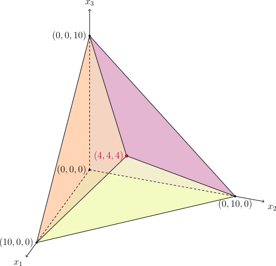
Geometrically, the solution process above corresponds to the following path between vertices of the polyhedron:

$$(0,0,0) \rightarrow (0,0,10) \rightarrow (10,0,0) \rightarrow (4,4,4).$$

Implementation Details

The simplex tableau can solve many linear programming problems. However, for the most general cases, the simplex method still has many details worth examining.

Slack Form

The method for converting a linear programming problem in general form to standard form was discussed above. To make it convenient to solve with the simplex method, we also need the coefficient matrix $A$ to have full rank. Although converting to standard form and then removing linearly dependent constraints works, the following strategy is usually used for simplicity:

1. Convert the linear programming problem to inequality form, namely $\min\{c^Tx : Ax \le b,~ x \ge 0\}$;
2. Add slack variables $s$ to obtain standard form: $\min\{c^Tx : Ax + s = b,~ x\ge 0,~ s \ge 0\}$.

The advantage is that the coefficient matrix $(A,I)$ of the resulting standard form is always full rank, and a (not necessarily feasible) basic solution $(x,s)=(0,b)$ always exists. This special standard form is called slack form.

Initial Basic Feasible Solution

The simplex method described above always assumes that a basic feasible solution is known. Sometimes one is easy to find. For example, if $b\ge 0$ in the slack form above, then $(x,s)=(0,b)$ is a basic feasible solution. This is the situation in the numerical example above.

For the general case, use the two-phase method. It performs the simplex method twice. The first phase solves a feasibility linear program and obtains a basic feasible solution of the original problem. The second phase starts from this basic feasible solution and applies the simplex method to solve the original problem.

Suppose the problem is in standard form $\min\{c^Tx : Ax = b \ge 0,~ x\ge 0\}$. In the first phase, solve

This is a feasibility linear program. The newly added variable $x_a$ is called an artificial variable. It has the basic feasible solution $(x,x_a)=(0,b)$, so it can be solved directly by the simplex method. If the optimum is strictly greater than $0$, then no $x\ge 0$ satisfies $Ax=b$, so the original problem is infeasible. If the optimum equals $0$, the artificial variables in an optimal solution must all be zero. If some artificial variables are still basic, pivot them out through several pivots. Finally, when all artificial variables are non-basic, the basic solution obtained in phase one can be used as the initial basic feasible solution for phase two.

The reference implementation is as follows:

Reference Implementation

// First phase: find an initial BFS.
// Return false if no feasible solution.
bool initialize() {
  int neg_count = 0;
  for (int j = 0; j < m; ++j) {
    if (tab[n][j] < -eps) {
      for (int i = 0; i <= n; ++i) {
        tab[i][m + 1] += tab[i][j];
      }
      B[j] = ~B[j];
      ++neg_count;
    }
  }
  while (neg_count) {
    int x = -1;
    long double mi = -eps;
    for (int i = 0; i < n; ++i) {
      if (tab[i][m + 1] < mi) {
        x = i;
        mi = tab[i][m + 1];
      }
    }
    if (x == -1) return false;
    int y = -1;
    mi = INFINITY;
    for (int j = 0; j < m; ++j) {
      if ((B[j] < 0 && tab[x][j] < -eps) || (B[j] >= 0 && tab[x][j] > eps)) {
        auto tmp = tab[n][j] / tab[x][j] + (B[j] < 0 ? -eps : eps);
        if (tmp < mi) {
          y = j;
          mi = tmp;
        }
      }
    }
    if (B[y] < 0) {
      --neg_count;
      B[y] = ~B[y];
      pivot(x, y);
      tab[x][m + 1] += 1;
    } else {
      pivot(x, y);
    }
  }
  return true;
}

Before phase one starts, add an extra row to record the phase-one objective function. During pivoting, pivot the entire tableau, including the phase-two objective function. Thus, when phase one is complete, the phase-two objective has also been updated accordingly, and phase two can begin directly with the simplex method.

The two-phase method can also be implemented with a single simplex method. Choose a sufficiently large positive number $M$ and directly solve

This yields the optimum of the original problem. In the implementation, $M$ is not assigned a concrete value; it is treated as an unknown sufficiently large positive number $M$. This method is called the big $M$ method.

// First phase: find an initial BFS.
// Return false if no feasible solution.
bool initialize() {
  while (true) {
    int y = -1;
    long double mi = -eps;
    for (int j = 0; j < m; ++j) {
      if (tab[n][j] <= mi) {
        y = j;
        mi = tab[n][j];
      }
    }
    // No row with a negative basic variable => Feasible.
    if (y == -1) break;
    int x = -1;
    for (int i = 0; i < n; ++i) {
      if (tab[i][y] < -eps && (x == -1 || N[i] > N[x])) {
        x = i;
      }
    }
    // No column with a negative entry => Infeasible.
    if (x == -1) return false;
    pivot(x, y);
  }
  return true;
}

Pivot Rules

During pivoting, if there are multiple choices for entering or leaving variables, use a pivot rule to choose which variables enter or leave. With a simplex tableau, every rule discussed here can find the entering and leaving variables in $O(mn)$ time, so one pivot still takes $O(mn)$ time.

The choice of entering variable often determines the number of pivots before termination. Common rules include:

• Choose the first entering variable found;
• Choose the entering variable with the smallest label (part of Bland's rule);
• Choose the entering variable with the largest absolute reduced cost (that is, $|c_i|$; Dantzig's rule);
• Choose the entering variable with the largest single-pivot improvement in the objective (that is, $|c_i|\theta_i$);
• Choose the entering variable corresponding to the steepest edge, namely the largest objective improvement per unit distance along the edge (that is, $|c_i|/\|A_B^{-1}A_i\|$);
• Choose an entering variable at random.

In practice, the steepest-edge rule is the most efficient². It is generally believed that a suitable pivot rule finds an optimal solution for most problems in roughly $2m$ pivots. However, every currently known pivot rule has specially constructed examples³ that force the number of pivots to be exponential. This is why the simplex method performs quite well in practice but has exponential worst-case complexity in theory.

The choice of leaving variable often determines whether the algorithm enters a cycle. If several basic feasible solutions have the same optimal value, the algorithm may cycle among them indefinitely. Such cases are uncommon, so many simplex implementations do not specify a rule for choosing the leaving variable. Two common anti-cycling rules are:

• Bland's rule: always choose the entering and leaving variables with the smallest labels.

• Lexicographic rule: always choose a row with $(A_B^{-1}A_i)_j>0$ and

  $$\left(\dfrac{(A_B^{-1}b)_j}{(A_B^{-1}A_i)_j},\dfrac{(A_B^{-1})_{j1}}{(A_B^{-1}A_i)_j},\cdots,\dfrac{(A_B^{-1})_{jm}}{(A_B^{-1}A_i)_j}\right)$$

  the leaving variable corresponding to the lexicographically smallest row index $j$, namely $x_{B_j}$. The choice of entering variable is unimportant.

  If the linear programming problem is in slack form, all these quantities can be obtained directly from the tableau $T_B$ described above. Otherwise, after finding an initial basic solution (not necessarily feasible), use the coefficients in the columns corresponding to the basic variables of this initial basis (with the order fixed) as the coefficients of $A_B^{-1}$.

Bland's rule is inefficient because it uses the same method to choose entering and leaving variables, which can easily cause the same variable to enter and leave repeatedly. The lexicographic rule is more practical. It is equivalent to perturbing the parameters of the linear programming problem⁴, so no two basic feasible solutions have the same optimal value and cycling is impossible.

Reference Implementation

This section provides a reference implementation of the two-phase simplex method based on the condensed simplex tableau.

#include <algorithm>
#include <climits>
#include <cmath>
#include <iomanip>
#include <iostream>
#include <numeric>
#include <vector>

// --8<-- [start:core]
int m, n;  // Number of constraints and variables.
std::vector<std::vector<long double>>
    tab;                             // Compressed tableau (transposed) with
                                     // first-phase objective attached.
std::vector<int> B, N;               // Basic and nonbasic variables.
constexpr long double eps = 1e-12l;  // Precision.

// --8<-- [start:pivot]
// Pivot on (N[x], B[y]).
void pivot(int x, int y) {
  std::swap(N[x], B[y]);
  long double v = -1 / tab[x][y];
  for (int j = 0; j <= m + 1; ++j) {
    tab[x][j] = j == y ? -v : v * tab[x][j];
  }
  for (int i = 0; i <= n; ++i) {
    if (i == x) continue;
    v = tab[i][y];
    tab[i][y] = 0;
    for (int j = 0; j <= m + 1; ++j) {
      tab[i][j] += v * tab[x][j];
    }
  }
}

// --8<-- [end:pivot]
// --8<-- [start:initialize]
// First phase: find an initial BFS.
// Return false if no feasible solution.
bool initialize() {
  int neg_count = 0;
  for (int j = 0; j < m; ++j) {
    if (tab[n][j] < -eps) {
      for (int i = 0; i <= n; ++i) {
        tab[i][m + 1] += tab[i][j];
      }
      B[j] = ~B[j];
      ++neg_count;
    }
  }
  while (neg_count) {
    int x = -1;
    long double mi = -eps;
    for (int i = 0; i < n; ++i) {
      if (tab[i][m + 1] < mi) {
        x = i;
        mi = tab[i][m + 1];
      }
    }
    if (x == -1) return false;
    int y = -1;
    mi = INFINITY;
    for (int j = 0; j < m; ++j) {
      if ((B[j] < 0 && tab[x][j] < -eps) || (B[j] >= 0 && tab[x][j] > eps)) {
        auto tmp = tab[n][j] / tab[x][j] + (B[j] < 0 ? -eps : eps);
        if (tmp < mi) {
          y = j;
          mi = tmp;
        }
      }
    }
    if (B[y] < 0) {
      --neg_count;
      B[y] = ~B[y];
      pivot(x, y);
      tab[x][m + 1] += 1;
    } else {
      pivot(x, y);
    }
  }
  return true;
}

// --8<-- [end:initialize]
// --8<-- [start:simplex]
// Second phase: find an optimal BFS.
// Return false if the problem is unbounded.
bool simplex() {
  while (true) {
    int x = -1;
    long double mi = -eps;
    for (int i = 0; i < n; ++i) {
      if (tab[i][m] < mi) {
        x = i;
        mi = tab[i][m];
      }
    }
    // No column with a negative reduced cost => Optimal.
    if (x == -1) break;
    int y = -1;
    mi = INFINITY;
    for (int j = 0; j < m; ++j) {
      if (tab[x][j] <= eps) continue;
      if (tab[n][j] / tab[x][j] < mi) {
        y = j;
        mi = tab[n][j] / tab[x][j];
      }
    }
    // No row with a positive ratio => Unbounded.
    if (y == -1) return false;
    pivot(x, y);
  }
  return true;
}

// --8<-- [end:simplex]
int solve() {
  B.resize(m);
  N.resize(n);
  std::iota(B.begin(), B.end(), n);
  std::iota(N.begin(), N.end(), 0);
  return initialize() ? (simplex() ? 0 : 1) : -1;
}

// --8<-- [end:core]
int main() {
  std::ios::sync_with_stdio(false), std::cin.tie(nullptr);
  std::cout << std::fixed << std::setprecision(8);
  std::cin >> n >> m;
  tab.assign(n + 1, std::vector<long double>(m + 2));
  for (int i = 0; i < n; ++i) {
    std::cin >> tab[i][m];
    tab[i][m] = -tab[i][m];
  }
  for (int j = 0; j < m; ++j) {
    for (int i = 0; i <= n; ++i) {
      std::cin >> tab[i][j];
    }
  }
  switch (solve()) {
    case -1:
      std::cout << "Infeasible" << std::endl;
      break;
    case 1:
      std::cout << "Unbounded" << std::endl;
      break;
    case 0: {
      std::cout << tab[n][m] << std::endl;
      std::vector<long double> x(n);
      for (int j = 0; j < m; ++j) {
        if (B[j] < n) x[B[j]] = tab[n][j];
      }
      for (int i = 0; i < n; ++i) {
        std::cout << x[i] << ' ';
      }
      std::cout << std::endl;
      break;
    }
  }
  return 0;
}

Examples

#include <cmath>
#include <cstring>
#include <iostream>
using namespace std;
constexpr int M = 10005, N = 1005, INF = 1e9;

int n, m;
double a[M][N], b[M], c[N], v;

void pivot(int l, int e) {  // function
  b[l] /= a[l][e];
  for (int j = 1; j <= n; j++)
    if (j != e) a[l][j] /= a[l][e];
  a[l][e] = 1 / a[l][e];

  for (int i = 1; i <= m; i++)
    if (i != l && fabs(a[i][e]) > 0) {
      b[i] -= a[i][e] * b[l];
      for (int j = 1; j <= n; j++)
        if (j != e) a[i][j] -= a[i][e] * a[l][j];
      a[i][e] = -a[i][e] * a[l][e];
    }

  v += c[e] * b[l];
  for (int j = 1; j <= n; j++)
    if (j != e) c[j] -= c[e] * a[l][j];
  c[e] = -c[e] * a[l][e];

  // swap(B[l],N[e])
}

double simplex() {
  while (true) {
    int e = 0, l = 0;
    for (e = 1; e <= n; e++)
      if (c[e] > (double)0) break;
    if (e == n + 1) return v;  // whenvnamelyis
    double mn = INF;
    for (int i = 1; i <= m; i++) {
      if (a[i][e] > (double)0 && mn > b[i] / a[i][e]) {
        mn = b[i] / a[i][e];  // fortheseeofl
        l = i;
      }
    }
    if (mn == INF) return INF;  // unbounded
    pivot(l, e);                // l,e
  }
}

int main() {
  cin.tie(nullptr)->sync_with_stdio(false);
  cin >> n >> m;
  for (int i = 1; i <= n; i++) cin >> c[i];
  for (int i = 1; i <= m; i++) {
    int s, t;
    cin >> s >> t;
    for (int j = s; j <= t; j++) a[i][j] = 1;  // denotestheikindsinjwhencan
    cin >> b[i];
  }
  cout << (int)(simplex() + 0.5);
}

Exercises

• Luogu P13337【modulo】
• UOJ#179.
• Luogu P4232 of
• Codeforces 1430 G. Yet Another DAG Problem
• AtCoder Beginner Contest 231 H - Minimum Coloring

References

• 【 + 】
• 2016
• algorithm
• Matoušek, Jiří, and Bernd Gärtner. Understanding and using linear programming. Vol. 1. Berlin: Springer, 2007.
• Inayatullah, Syed, Nasir Touheed, and Muhammad Imtiaz. "A streamlined artificial variable free version of simplex method." PloS one 10, no. 3 (2015): e0116156.
• Floudas, Christodoulos A., and Panos M. Pardalos, eds. Encyclopedia of optimization. Springer Science & Business Media, 2008.