Stern–Brocot Trees and Farey Sequences

Introduction

This article introduces a data structure for storing reduced fractions and other related concepts. They are closely related to continued fractions, can be used to solve a series of number-theory problems in algorithmic competitions, and may appear as implicit background in some problems.

Stern–Brocot tree

The Stern–Brocot tree is an elegant structure for maintaining fractions, containing all distinct positive rational numbers. This structure was discovered independently by Moritz Stern in 1858 and Achille Brocot in 1861.

Construction

Layer-by-layer construction

The Stern–Brocot tree can be obtained while iteratively constructing the Stern–Brocot sequence of order $k$ (Stern–Brocot sequence of order $k$). The Stern–Brocot sequence of order $0$ consists of two simple fractions:

Strictly speaking, $\dfrac{1}{0}$ is not a rational fraction; it can be understood as the reduced fraction representing $\infty$.

For two adjacent fractions $\dfrac{a}{b}$ and $\dfrac{c}{d}$ in the Stern–Brocot sequence of order $k$, insert their mediant¹ $\dfrac{a+c}{b+d}$ between them to obtain the Stern–Brocot sequence of order $k+1$. Although the definition of the mediant itself allows fractions to be reduced, in constructing the Stern–Brocot tree it is enough to add the numerators and denominators directly, without worrying about reduction. Thus, Stern–Brocot sequences of all orders can be constructed iteratively. The results of the first few iterations are as follows:

Connecting the fractions newly added at each iteration into a tree structure gives the Stern–Brocot tree, as shown below:

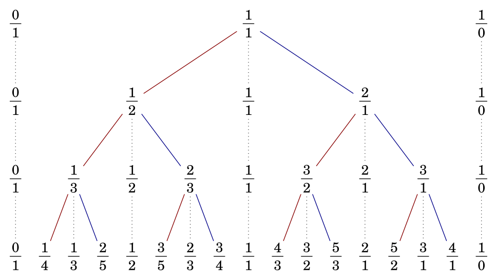
Excluding its left and right endpoints, the Stern–Brocot sequence of order $k$ is the in-order traversal of the Stern–Brocot tree at depth $k-1$.

Triple construction

Another equivalent construction uses triples.

Take this as the root node, and for every node

add

as its left and right child, respectively, to construct the entire Stern–Brocot tree. In the triple recorded by each node of the Stern–Brocot tree, the fraction actually stored is the middle fraction $\dfrac{p}{q}$; the two fractions $\dfrac{a}{b}$ and $\dfrac{c}{d}$ on either side appeared earlier. Moreover, considering the first construction shows that the fraction $\dfrac{p}{q}$ is obtained precisely by inserting the mediant of $\dfrac{a}{b}$ and $\dfrac{c}{d}$.

Matrix representation and the Stern–Brocot number system

The triple construction means that every node in the Stern–Brocot tree corresponds to a matrix

The root node of the Stern–Brocot tree is the identity matrix $I$. Moving to the left child and moving to the right child correspond respectively to right-multiplying the current node matrix by

The fraction actually corresponding to each node is $f(S)=\dfrac{a+c}{b+d}$. The matrix $S$ of each node can be written as a product of a sequence of matrices $L$ and $R$, which can also be viewed as a string formed from $L$ and $R$ representing the path from the root to that node. Uniquely representing every positive rational number by such a string can be regarded as a representation of positive rational numbers, and is therefore also called the Stern–Brocot number system.

Tree construction implementation

The tree-construction algorithm only needs to simulate the process above. The following code performs an in-order traversal of the first $n$ layers of the Stern–Brocot tree.

// In-Order Transversal of Stern-Brocot Tree till Layer N.
void build(int n, int a = 0, int b = 1, int c = 1, int d = 0, int level = 1) {
  if (level > n) return;  // Only first n layers.
  int x = a + c, y = b + d;
  build(n, a, b, x, y, level + 1);
  std::cout << x << '/' << y << ' ';  // Output the current fraction.
  build(n, x, y, c, d, level + 1);
}

# In-Order Transversal of Stern-Brocot Tree till Layer N.
def build(n, a=0, b=1, c=1, d=0, level=1):
    if level > n:
        return
    x, y = a + c, b + d
    build(n, a, b, x, y, level + 1)
    print(f"{x}/{y}", end=" ")
    build(n, x, y, c, d, level + 1)

The complexity of the tree-construction algorithm is $O(n^2)$.

Properties

We next discuss properties of the Stern–Brocot tree. In brief, the Stern–Brocot tree is a binary search tree containing all positive reduced rational fractions; it is also a heap of numerators and denominators, and a Cartesian tree of pairs formed by denominators and numerators. If the intervals formed by the left and right endpoints in the triple construction above are considered, the Stern–Brocot tree can also be regarded as a segment tree over $[0,\infty]$. These statements follow from the three basic properties below.

Monotonicity

In the construction above, the fractions in every layer are monotonically increasing. This only requires an inductive proof. If $\dfrac{a}{b} < \dfrac{c}{d}$, then necessarily

This follows by clearing the denominators in the inequalities. The induction starts from $\dfrac{0}{1} < \dfrac{1}{0}$, where monotonicity is also obvious.

Reducedness

In the construction above, every fraction is reduced. Again, inductively prove that every pair of adjacent fractions $\dfrac{a}{b}$ and $\dfrac{c}{d}$ in each layer of the construction satisfies

At the root node this is true because the matrix is the identity matrix. When moving downward, the matrices $L$ and $R$ being multiplied in have determinant $1$, so by the properties of the determinant, the same holds in the next layer:

This is also obvious for the induction starting pair $\dfrac{0}{1}$ and $\dfrac{1}{0}$. Therefore, by Bézout's identity, the numerator and denominator of every fraction are necessarily coprime; all fractions are thus reduced.

Completeness

Finally, we need to show that the Stern–Brocot tree contains all positive reduced fractions. The first two properties already show that the Stern–Brocot tree is a binary search tree, and any positive reduced fraction $\dfrac{p}{q}$ must lie between $\dfrac{0}{1}$ and $\dfrac{1}{0}$. By the method of searching a binary search tree, the only way for $\dfrac{p}{q}$ not to occur in the binary search tree would be for the search process to continue forever. This is impossible.

Suppose that we already know

then necessarily

Multiplying the two inequalities by $(c+d)$ and $(a+b)$ respectively gives

Using the equality $bc-ad=1$ established above, we obtain

Every time the search goes one level deeper, the right-hand side strictly increases while the left-hand side remains unchanged, so the search must stop after finitely many steps.

Finding fractions

In practical applications of the Stern–Brocot tree, it is often necessary to query the position of a given fraction in the tree.

Naive algorithm

Since the Stern–Brocot tree is a binary search tree, comparing the current fraction with the fraction being sought is enough to determine the path from the root to the given fraction. Denote moving to a left child and moving to a right child along the path by $L$ and $R$, respectively. Each path then corresponds to a string formed from $L$ and $R$, which is the representation of a rational number in the Stern–Brocot number system mentioned above. Finding the path to a rational number is equivalent to finding its representation in the Stern–Brocot number system.

The naive fraction-search algorithm is implemented as follows:

// Locate a given fraction in the Stern-Brocot tree.
std::string find(int x, int y, int a = 0, int b = 1, int c = 1, int d = 0) {
  int m = a + c, n = b + d;
  if (x == m && y == n) return "";
  if (x * n < y * m) {
    return 'L' + find(x, y, a, b, m, n);
  } else {
    return 'R' + find(x, y, m, n, c, d);
  }
}

# Locate a given fraction in the Stern-Brocot tree.
def find(x, y, a=0, b=1, c=1, d=0):
    m = a + c
    n = b + d
    if x == m and y == n:
        return ""
    if x * n < y * m:
        return "L" + find(x, y, a, b, m, n)
    else:
        return "R" + find(x, y, m, n, c, d)

The algorithm has complexity $O(p+q)$, so it is not practical in algorithmic competitions.

In the Stern–Brocot number system, every positive irrational number corresponds to a unique infinite string. The same algorithm can be used to construct this string. Every prefix of the infinite string corresponds to a rational reduced fraction. If these reduced fractions are arranged in a sequence, the denominators of the fractions are strictly increasing, and the limit of the sequence is the irrational number. Therefore, the Stern–Brocot tree can be used to find a rational approximation of any desired precision for an irrational number. However, note that the difference between this sequence of rationals and the irrational number is not strictly decreasing. For a strict theory of rational approximation, refer to the section on Diophantine approximation on the continued-fractions page. In practical applications of the Stern–Brocot tree to find the best approximation to a real number with denominator bounded by some range, one should finally remember to compare the distances from the two interval endpoints to that real number.

Fast algorithm

The naive fraction-search algorithm is not very efficient, but a simple optimization yields a fast search algorithm with complexity $O(\log(p+q))$. The key is to process consecutive $L$'s and $R$'s together.

If the fraction $\dfrac{p}{q}$ being sought lies between $\dfrac{a}{b}$ and $\dfrac{c}{d}$, then after moving right $t$ consecutive times, the right boundary remains fixed and the left node moves to $\dfrac{a+tc}{b+td}$; conversely, after moving left $t$ consecutive times, the left boundary remains fixed and the right node moves to $\dfrac{ta+c}{tb+d}$. Thus, the numbers of moves right and left can be determined directly using $\dfrac{a+tc}{b+td}<\dfrac{p}{q}$ or $\dfrac{p}{q}<\dfrac{ta+c}{tb+d}$. Strict inequalities are used here because the algorithm moves the left and right endpoints, while the fraction being sought appears as the mediant of the final endpoints.

// Locate a given fraction in the Stern-Brocot tree.
auto find(int x, int y) {
  std::vector<std::pair<int, char>> res;
  int a = 0, b = 1, c = 1, d = 0;
  bool right = true;
  while (x != a + c || y != b + d) {
    if (right) {
      auto t = (b * x - a * y - 1) / (y * c - x * d);
      res.emplace_back(t, 'R');
      a += t * c;
      b += t * d;
    } else {
      auto t = (y * c - x * d - 1) / (b * x - a * y);
      res.emplace_back(t, 'L');
      c += t * a;
      d += t * b;
    }
    right ^= 1;
  }
  return res;
}

# Locate a given fraction in the Stern-Brocot tree.
def find(x, y):
    res = []
    a, b, c, d = 0, 1, 1, 0
    right = True
    while x != a + c or y != b + d:
        if right:
            t = (b * x - a * y - 1) // (y * c - x * d)
            res.append((t, "R"))
            a += t * c
            b += t * d
        else:
            t = (y * c - x * d - 1) // (b * x - a * y)
            res.append((t, "L"))
            c += t * a
            d += t * b
        right ^= 1
    return res

The current search algorithm requires the fraction $\dfrac{p}{q}$ to be known. If the target fraction is unknown, the number of moves at each step right or left often needs to be found by exponential search or binary search. The complexity of the fraction-search algorithm is then $O(\log^2(p+q))$.

Continued-fraction-based algorithm

When the fraction is known, continued fractions give a simpler algorithm. Without loss of generality, assume that the first group of moves is to the right; otherwise, set the number of rightward moves in the first group to zero. Move the endpoints alternately right and left, and list the endpoint positions after each group of moves as follows:

Even-numbered groups move right, so they record the position of the left endpoint; odd-numbered groups move left, so they record the position of the right endpoint. Prepend two more endpoints to this list:

Let the number of moves in group $k$ be $t_k$. From the relationship between the numbers of moves and endpoint positions above, we have

The recurrence relation for continued fractions then gives

The final result is

Therefore, in the simple continued-fraction representation of the target fraction whose final term is one, excluding the final one, the preceding terms encode the path from the root to the current node in the Stern–Brocot tree. Even-indexed terms, with indices starting at $0$, are edges to right children, and odd-indexed terms are edges to left children.

A rational number's continued-fraction representation can be obtained by the Euclidean algorithm, so the continued-fraction-based fraction-search algorithm has complexity $O(\log\min\{p,q\})$.

// Locate a given fraction in the Stern-Brocot tree.
auto find(int x, int y) {
  std::vector<std::pair<int, char>> res;
  bool right = true;
  while (y) {
    res.emplace_back(x / y, right ? 'R' : 'L');
    x %= y;
    std::swap(x, y);
    right ^= 1;
  }
  --res.back().first;
  return res;
}

# Locate a given fraction in the Stern-Brocot tree.
def find(x, y):
    res = []
    right = True
    while y:
        res.append([x // y, ("R" if right else "L")])
        x, y = y, x % y
        right ^= 1
    res[-1][0] -= 1
    return res

The continued-fraction representation also gives a simple way to express the parent and children of a node. For the node $[t_0,t_1,\cdots,t_n,1]$, its parent is the node that moves one fewer step in the final direction: when $t_k>1$, the parent is $[t_0,t_1,\cdots,t_n - 1,1]$; otherwise, the parent is $[t_0,t_1,\cdots,t_{n-1},1]$. Its two children are $[t_0,t_1,\cdots,t_n+1,1]$ and $[t_0,t_1,\cdots,t_n,1,1]$, respectively. Which of the two nodes is the left child and which is the right child depends on the parity of $n$.

Calkin–Wilf tree

Another, simpler structure for storing positive rational fractions is the Calkin–Wilf tree. It is usually shown as follows:

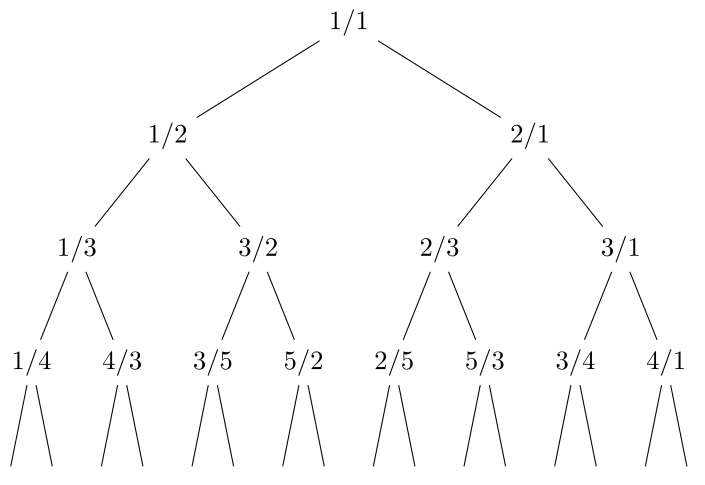
The root node is $\dfrac{1}{1}$. For the node containing the fraction $\dfrac{p}{q}$, its left and right children are $\dfrac{p}{p+q}$ and $\dfrac{p+q}{q}$, respectively. Like the Stern–Brocot tree, every fraction in it is reduced, and it contains every positive reduced fraction exactly once.

Relation to continued fractions

Unlike the Stern–Brocot tree, the Calkin–Wilf tree is not a binary search tree, so it cannot be used to perform binary searches for rational numbers.

In the Calkin–Wilf tree, when $p>q$, the parent of the node containing $\dfrac{p}{q}$ is $\dfrac{p-q}{q}$; when $p<q$, it is $\dfrac{p}{q-p}$. In the first case, starting from $\dfrac{p}{q}$, the node is the right child of its parent. We can keep moving upward through the right side of the parent until the numerator is no longer greater than the denominator. The fraction stored at that point is $\dfrac{p\bmod q}{q}$, and the number of moves in this group is $\left\lfloor\dfrac{p}{q}\right\rfloor$. In the second case, it is the left child of its parent. We can keep moving upward through the left side of the parent until the denominator is no longer greater than the numerator. The fraction stored then is $\dfrac{p}{q\bmod p}$, and the number of moves in this group is $\left\lfloor\dfrac{q}{p}\right\rfloor$.

In the language of continued fractions, suppose the current node stores a remainder $s_k$ of a continued fraction. Moving upward along the right side of the parent $\lfloor s_k\rfloor$ times reaches the fraction $\dfrac{1}{s_{k+1}}$, after which moving upward along the left side of the parent $\lfloor s_{k+1}\rfloor$ times reaches the fraction $s_{k+2}$. Therefore, starting from node $s_0=\dfrac{p}{q}$ and moving upward to the root node $\dfrac{1}{1}$, the path is encoded by the continued fraction $[t_0,t_1,\cdots,t_n,1]$: excluding the final $1$, even-indexed terms, with indices starting at $0$, give the number of upward moves along the right side of the parent, and odd-indexed terms give the number of upward moves along the left side.

For the node containing the fraction $\dfrac{p}{q}=[t_0,t_1,\cdots,t_n,1]$, its parent has the following representations:

1. When $t_0>0$, its parent is $\dfrac{p-q}{q}=[t_0 - 1, t_1, \cdots, t_n,1]$;
2. When $t_0=0$ and $t_1>1$, its parent is $\dfrac{p}{q-p} = [0, t_1 - 1, t_2, \cdots, t_n,1]$;
3. When $t_0=0$ and $t_1=1$, its parent is $\dfrac{p}{q-p} = [t_2, t_3, \cdots, t_n,1]$.

Conversely, its children are $\dfrac{p+q}{q}=[t_0+1,t_1,\cdots,t_n,1]$ and $\dfrac{p}{p+q}=[0,1,t_0,t_1,\cdots,t_n,1]$, respectively. For the continued-fraction representation of the second child, when $t_0=0$, it should be understood as $[0,1+t_1,\cdots,t_n,1]$.

Relation to the Stern–Brocot tree

As with continued fractions, the nodes along a path in the Stern–Brocot tree exhibit the recurrence relation of convergents, while the nodes along a path in the Calkin–Wilf tree exhibit the recurrence relation of remainders. The continued-fraction representation of a given fraction is fixed, so the encoding of its path to the root in the Calkin–Wilf tree and the encoding of the path from the root to it in the Stern–Brocot tree are exactly the same. However, because the path directions are reversed, although the fractions stored at the same level of the Stern–Brocot tree and the Calkin–Wilf tree are the same, their positions are different.

If both trees are traversed by breadth-first search and nodes are numbered in order, with the root numbered $1$, then the left and right children of node $v$ are $2v$ and $2v+1$. Looking at the binary representation of the number, after removing the initial $1$, each $1$ from the most significant bit to the least significant bit represents moving to a right child, and each $0$ represents moving to a left child. In the Calkin–Wilf tree, the number of the node containing the rational number represented by $[t_0,t_1,\cdots,t_n,1]$ is

Correspondingly, in the Stern–Brocot tree, the number of the node containing the rational number represented by $[t_0,t_1,\cdots,t_n,1]$ is

After removing the initial $1$, the remaining bits form exactly the left-to-right numbering of the vertices at the same level, starting from $0$. This derivation shows that the order of the fractions at the same level in the Stern–Brocot tree and the Calkin–Wilf tree are related by a bit-reversal permutation: reverse the binary bits of the index, padding with the initial $0$, to obtain the permutation on $0\sim (2^k-1)$.

For this reason, nodes in the Stern–Brocot tree are sometimes numbered according to their corresponding node numbers in the Calkin–Wilf tree, producing the numbering shown below:

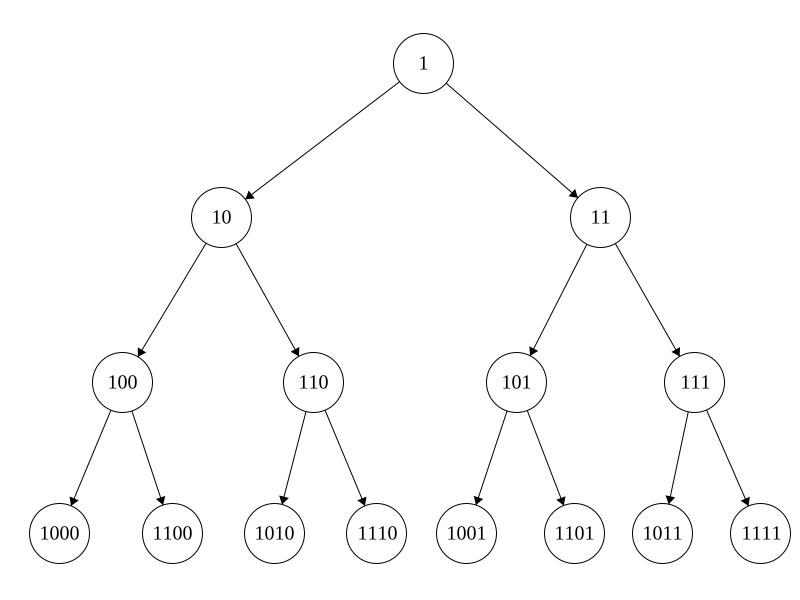
This numbering can be constructed recursively: the root node is numbered $1$; whenever moving to a left child, replace the leading $1$ of the number with $10$, and whenever moving to a right child, replace the leading $1$ with $11$. Reading this number from right to left gives the path from the root to the node.

Stern's diatomic sequence

Ordering all fractions in the Calkin–Wilf tree by their breadth-first-search numbers, or ordering all fractions in the Stern–Brocot tree by the numbers shown above, gives the following sequence:

The construction of the Calkin–Wilf tree proves that, in this sequence, the denominator of each fraction is necessarily equal to the numerator of the next fraction. Listing the numerators alone gives Stern's diatomic sequence (Stern diatomic sequence, OEIS A002487), also called the Stern–Brocot sequence. The sequence above is numbered starting from $1$, with the additional convention that its $0$th term is $0$.

Let $a_n$ be the $n$th term of Stern's diatomic sequence. It satisfies the following recurrence:

The recurrence starts from $a_0=0$ and $a_1=1$. Directly using the recurrence to obtain $a_n$ has complexity $O(\log^2n)$, which is not ideal. A better approach is to regard it as the numerator of the fraction at node $n$ in the Calkin–Wilf tree and solve it using the continued-fraction recurrence described above, with complexity $O(\log n)$.

Farey sequence

Farey sequences have characteristics extremely similar to those of the Stern–Brocot tree. Let the Farey sequence of order $n$ (Farey sequence of order $n$) be denoted by $F_n$. It is the sequence formed by arranging in increasing order all reduced fractions between $[0,1]$ whose denominators are at most $n$:

By definition, Farey sequences naturally satisfy monotonicity, reducedness, and completeness. As shown above, the fractions newly added to $F_k$ relative to $F_{k-1}$ are always the mediants of adjacent fractions in $F_{k-1}$.

The algorithm for constructing the Stern–Brocot tree above also applies to constructing Farey sequences. Since the Stern–Brocot tree contains all reduced fractions, changing only the boundary condition to constrain the denominator gives code for constructing a Farey sequence. The Farey sequence of order $n$, $F_n$, can be regarded as a subsequence of the Stern–Brocot sequence of order $n-1$.

// Farey Sequence of Order N.
void build(int n, int a = 0, int b = 1, int c = 1, int d = 1,
           bool init = true) {
  int x = a + c, y = b + d;
  if (y > n) return;              // Only first n layers.
  if (init) std::cout << "0/1 ";  // Output 0/1;
  build(n, a, b, x, y, false);
  std::cout << x << '/' << y << ' ';  // Output the current fraction.
  build(n, x, y, c, d, false);
  if (init) std::cout << "1/1 ";  // Output 1/1;
}

# Farey Sequence of Order N.
def build(n, a=0, b=1, c=1, d=1, init=True):
    x, y = a + c, b + d
    if y > n:
        return
    if init:
        print("0/1", end=" ")
    build(n, a, b, x, y, False)
    print(f"{x}/{y}", end=" ")
    build(n, x, y, c, d, False)
    if init:
        print("1/1", end=" ")

The complexity of directly constructing a Farey sequence is $O(|F_n|)=O(n^2)$.

Sequence length and fraction search

The length of a Farey sequence can be obtained recursively. Relative to $F_{n-1}$, the additional fractions in $F_n$ all have denominator $n$, and their numerators are at most $n$ and coprime to $n$. Therefore,

Here $\varphi(n)$ is the Euler totient function. The expression can be evaluated in $O(n)$ using the linear sieve, or its complexity can be reduced to $O(n^{2/3})$ using the Du sieve.

More commonly than finding the length directly, we need to find the index of a fraction $r=\dfrac{p}{q}$ in the sequence $F_k$. This amounts to evaluating

Mobius inversion was used to obtain the right-hand side. Combining the linear sieve with factor enumeration gives $O(n)$ preprocessing and $O(n\log n)$ per query; combining the Du sieve with the Euclidean-like algorithm gives $O(n^{2/3})$ preprocessing and $O(\sqrt n\log n)$ per query.

Conversely, solving for the fraction from a known index requires binary-searching the real numbers between $[0,1]$, or performing a binary search on the Stern–Brocot tree. The former may be limited by floating-point precision and takes $O(\log V)$ fraction-index queries, where $V$ is the precision range; the latter is not limited by floating-point precision but takes $O(\log^2n)$ fraction-index queries.

Farey neighbors

If the fractions $\dfrac{a}{b}$ and $\dfrac{c}{d}$ are adjacent in some Farey sequence, they are called Farey neighbors, also called a Farey pair.

Let $\dfrac{a}{b}<\dfrac{c}{d}$. From the construction of Farey sequences, the fraction added later among two adjacent fractions is necessarily the mediant of the other fraction and its earlier neighbor. Therefore, Farey neighbors are also adjacent in a Stern–Brocot sequence of some order. By the result proved in Reducedness, we necessarily have

Conversely, this is also a sufficient condition for two reduced proper fractions to be Farey neighbors. To see this, suppose without loss of generality that $\dfrac{a}{b}$ is the fraction with the larger denominator. Both fractions then appear in $F_b$. Let $\dfrac{e}{f}$ be the term immediately to the right of $\dfrac{a}{b}$ in $F_b$. By the necessity already shown, $be-af=1$. However, the linear congruence equation $bx-ay=1$ has only one positive integer solution with $y\le b$, so necessarily $(e,f)=(c,d)$.

In fact, because the next reduced fraction to appear between the two must be $\dfrac{a+c}{b+d}$, the fractions $\dfrac{a}{b}$ and $\dfrac{c}{d}$ are adjacent in every Farey sequence from order $\max\{b,d\}$ through order $(b+d-1)$.

The Farey-neighbor relation for denominators at most $9$ is shown below:

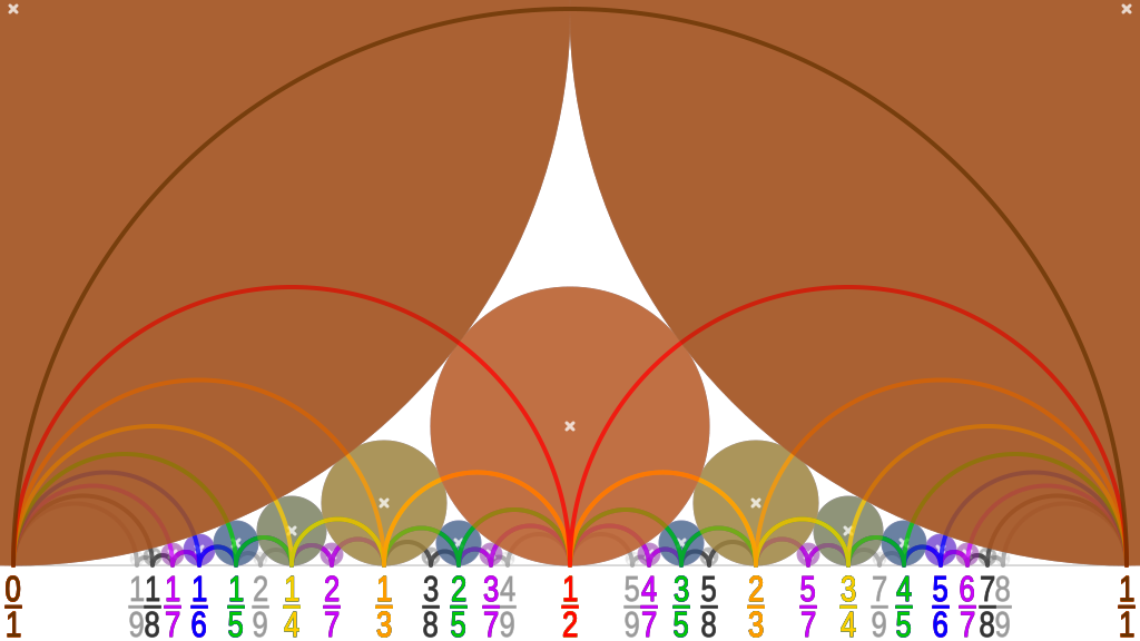
The circles in the figure are called Ford circles: for every reduced fraction $\dfrac{p}{q}$ in $[0,1]$, draw a circle centered at $\left(\dfrac{p}{q},\dfrac{1}{2q^2}\right)$ with radius $\dfrac{1}{2q^2}$. The figure shows that the Ford circles corresponding to two fractions can only be tangent or disjoint, and the two circles are tangent if and only if the fractions are Farey neighbors. Moreover, for any two tangent circles in the figure, there is always a unique third circle tangent to both. This third circle corresponds to the mediant of the fractions corresponding to the two circles.

To verify that tangent circles always correspond to Farey neighbors, directly compute the distance between their centers:

Since the two reduced fractions are distinct, $|bc-ad|\ge 1$, so the two circles can only be tangent or disjoint. Moreover, the circles are tangent if and only if $|bc-ad|=1$, which is equivalent to the fractions being Ford neighbors.

Finally, we count the number of Farey-neighbor pairs. Apart from $\left(\dfrac{0}{1},\dfrac{1}{1}\right)$, the denominators of the other Farey neighbors are different. Suppose without loss of generality that $\dfrac{p}{q}$ is the one with the larger denominator. The other fraction can necessarily be obtained by solving the binary linear Diophantine equation

Each of the two equations has exactly one positive integer solution satisfying $y<q$, corresponding respectively to the neighbor on the left and on the right of $\dfrac{p}{q}$. Thus every proper fraction in $(0,1)$ has two Farey neighbors with smaller denominators; adding $\dfrac{0}{1}$ and $\dfrac{1}{1}$ shows that $F_n$ contains $(2|F_n|-3)$ Farey-neighbor pairs in total.

Of course, the fraction $\dfrac{a}{b}<\dfrac{c}{d}$ found in this process is the left and right neighbor of $\dfrac{p}{q}$ when it is inserted into the sequence. They are therefore already Farey neighbors, and $\dfrac{p}{q}$ is their mediant. Let $\dfrac{p}{q}=[t_0,t_1,\cdots,t_n,1]$. Then the two Farey neighbors with smaller denominators are $[t_0,t_1,\cdots,t_n]$ and $[t_0,t_1,\cdots,t_{n-1}]$, respectively.

To compute the other Farey neighbors of the current fraction $\dfrac{p}{q}$, it is enough to use the extended Euclidean algorithm to find all solutions satisfying the conditions.

Recurrence relation

Farey sequences have a simple recurrence relation that can be used to obtain all fractions in the Farey sequence of order $n$ from left to right.

First, the preceding analysis shows that in $F_n$, every newly added term $\dfrac{p}{n}$ is always the mediant of two adjacent fractions. In fact, this relation holds for every fraction in $F_n$ except the two endpoints. Let $\dfrac{a}{b}<\dfrac{p}{q}<\dfrac{c}{d}$. By the necessary and sufficient condition for Farey neighbors, we always have

In the general case, however, the fraction $\dfrac{a+c}{b+d}$ may need to be reduced.

This observation gives the following recurrence relation. Suppose $\dfrac{a}{b}$ and $\dfrac{p}{q}$ are known, and we want to find the value of the third fraction $\dfrac{c}{d}$. There is then a $k$ such that

holds. Because the difference

decreases as $k$ increases, and the fraction immediately adjacent to $\dfrac{p}{q}$ should be the one with the smallest such difference among all fractions satisfying $kq-d\le n$, we necessarily have

It can be verified that the fraction obtained in this way is necessarily in $F_n$. Therefore, the numerators and denominators of fractions in $F_n$ satisfy the recurrence

The recurrence starts from $(p_0,q_0)=(0,1)$ and $(p_1,q_1)=(1,n)$.

Exercises

Problems based on the material in this article:

• LOJ 6685. Maze
• UVa 10077. The Stern-Brocot Number System
• Luogu P8058. [BalkanOI2003] Farey sequence
• UVa 12995. Farey Sequence
• UVa 10408. Farey Sequences
• UVa 12438. Farey Polygon
• AtCoder ARC123F. Insert Addition

Problems requiring binary search on the Stern–Brocot tree:

• AtCoder ABC333G. Nearest Fraction
• SPOJ DIVCNT1 - Counting Divisors
• SPOJ AFS3 - Amazing Factor Sequence (hard)

References and notes

• Stern–Brocot tree - Wikipedia
• Calkin–Wilf tree - Wikipedia
• Farey sequence - Wikipedia

Some content on this page is translated from the blog post Дерево Штерна-Броко. Ряд Фарея and its English translation The Stern-Brocot Tree and Farey Sequences. The Russian version is licensed under Public Domain + Leave a Link; the English version is licensed under CC-BY-SA 4.0. Some other content on this page is translated from the blog post Continued fractions, licensed under CC-BY-SA 4.0. The content has been modified.