Introduction
Continued fractions can represent a real number as the limit of a convergent sequence of rational numbers. The rational numbers in this sequence are easy to compute and provide the best approximations to the real number, so continued fractions are often used in algorithmic competitions. In addition, continued fractions are closely related to the Euclidean algorithm and can therefore be applied to a series of number-theoretic problems.
Implementing continued-fraction algorithms
This article provides implementations of a series of continued-fraction algorithms. Some algorithms may not guarantee that the integers involved in intermediate computations fit within 32-bit or 64-bit integer variables. In such cases, refer to the corresponding Python implementation, or replace the integer variables in the C++ implementation with a big integer class. To keep the focus on the main ideas, some code in this article may call functions implemented earlier without repeating their implementations.
Continued fractions
A continued fraction (continued fraction) is, in itself, only a form of notation.
Finite continued fractions
For a sequence , the continued fraction denotes the expansion
A continued fraction is meaningful if and only if the corresponding expansion is meaningful. These are called the terms or coefficients of the continued fraction.
Notation
More general continued fractions allow the numerators in the expansion to be other than , which requires modifying the notation accordingly; this is beyond the scope of this article. In addition, some literature writes the first comma “” as a semicolon “”; this has no difference in meaning from the notation used here.
Of course, continued fractions can also be generalized to infinite sequences.
Infinite continued fractions
For an infinite sequence , the continued fraction denotes the limit
A continued fraction is meaningful if and only if the corresponding limit is meaningful. Here, is called the convergent of with index , while is called the remainder or complete quotient of with index . Accordingly, the term is sometimes called the -th partial quotient.
Simple continued fractions
In number theory, we mainly consider the case where all terms of a continued fraction are integers.
Simple continued fractions
For a continued fraction , if is an integer and are all positive integers, it is called a simple continued fraction, also abbreviated as a continued fraction. If the sequence is finite, it is called a finite (simple) continued fraction; otherwise, it is called an infinite (simple) continued fraction. In addition, is called its integer part.
Unless otherwise stated, every continued fraction mentioned in this article means a simple continued fraction. It can be proved that every infinite simple continued fraction converges, and its remainders are always positive.
Continued fractions have the following basic properties:
Properties
Let be a real number. Then the following properties hold:
- For any , ;
- For a real number , , and its reciprocal is .
Finite continued fractions correspond to rational numbers. Every rational number has exactly two representations as a continued fraction, whose lengths necessarily have opposite parity. The only difference between the two representations is whether the last term is , namely
These two continued fractions are called the continued fraction representations of the rational number . The one whose final term is not one is called the standard representation, and the one whose final term is one is called the nonstandard representation.1
Example
The continued fraction representations of the rational number are
Infinite continued fractions correspond to irrational numbers. Moreover, every irrational number has exactly one representation as a continued fraction, called its continued fraction representation.
Finding a continued-fraction representation
To find the continued fraction representation of a real number , observe that if its remainder is not an integer, then it necessarily satisfies
Also, . Therefore, starting from , we can recursively compute
The sequence produced by this process is always uniquely determined, unless some remainder becomes an integer. If is an integer, the process should terminate, and we may choose to output either the corresponding standard or nonstandard representation.
In algorithmic competitions, we often handle rational numbers . Here, every remainder is a rational number , and for , since , we always have . Computing the recurrence above gives
The computation is in fact applied to and using the Euclidean algorithm. This also shows that for a rational number , the length of its continued fraction representation is , and the complexity of computing the continued fraction of is also .
Reference implementation
Given the numerator and denominator of a fraction, output the coefficient sequence of its continued fraction.
C++
// Find the continued fraction representation of P/Q.
auto fraction(int p, int q) {
  std::vector<int> a;
  while (q) {
    a.push_back(p / q);
    std::tie(p, q) = std::make_pair(q, p % q);
  }
  return a;
}
Python
# Find the continued fraction representation of P/Q.
def fraction(p, q):
    a = []
    while q:
        a.append(p // q)
        p, q = q, p % q
    return a
Convergents
The concept of convergents was introduced in the definition of continued fractions. For a real number , retaining the first terms of its continued fraction representation gives the continued fraction , which is called a convergent of with index . Every convergent of , including , is rational, and the sequence converges to .
Example: convergents of the golden ratio
The first few convergents of the continued fraction are
By induction, we can prove
where is the Fibonacci sequence. Its closed form gives
where is the golden ratio. As tends to infinity,
Therefore, the continued fraction represents the golden ratio .
These convergents approach the corresponding real number, so they can be used to approximate it. For this purpose, we need to understand the properties of convergents.
Recurrence
First, we need to solve the problem of computing these convergents. Although a convergent is obtained by appending one term to the continued fraction, it is not necessary to recompute its value each time. In fact, convergents satisfy the following recurrence:
Recurrence formula
For a continued fraction , suppose its -th convergent can be written as the fraction . Then
The recurrence starts from the (formal) fractions
Proof
The numerator and denominator of the convergent can be viewed as multivariate polynomials in :
By the definition of a convergent,
Comparing this with the preceding expression, set without loss of generality. Then the convergent can be written as
and the polynomial satisfies the recurrence
Since
the starting values are
If we set
it can be verified that the recurrence also holds for . This is equivalent to defining the formal fractions and .
The polynomial sequence satisfying the recurrence above is called the continuant2. It can be written in determinant form:
This is the determinant of a tridiagonal matrix. Expanding from the upper-left corner verifies that it satisfies the recurrence and initial conditions above. Conversely, expanding from the lower-right corner gives the recurrence
which is what we needed to prove.
Notation
When this article writes the convergent as , it always means that the numerator and denominator are given by the recurrence above. We will show below that this always produces the reduced form of the convergent.
The recurrence shows that
lies between and .
As corollaries of the recurrence for convergents, we have the following reversal and reciprocal theorems:
Reversal theorem
Suppose the real number has a convergent with index , namely . Then the ratios of the numerators and denominators of two adjacent convergents are respectively
If =0, interpret the first continued fraction as truncated at the penultimate term, namely .
Proof
Dividing the two sides of the recurrences for and by and respectively gives
Iterating these two equations gives two continued fractions. Substituting the initial values and completes the result. When , interpret the resulting continued fraction as a formal expression; its remainder is
Thus, the last two terms can be omitted directly. For a rigorous proof, simply observe that this expression can be regarded as the limit as .
Reciprocal theorem
The reciprocal of a convergent of a real number is a convergent of .
Proof
Without loss of generality, let and let its continued fraction representation be . Then the continued fraction representation of is . Their convergents can be obtained from the recurrence. For , the initial conditions are and ; for , the initial conditions are and . Therefore, and . The recurrence gives . This shows that the reciprocals of the convergents of are convergents of . The case can be discussed similarly.
Using the recurrence obtained in this section, we get the following algorithm for computing convergents:
Reference implementation
Given the coefficients of a continued fraction, find the sequences of numerators and denominators of its convergents.
C++
// Find the convergents of a continued fraction A.
// Numerators and denominators stored separately in P and Q.
auto convergents(std::vector<int> a) {
  std::vector<int> p = {0, 1};
  std::vector<int> q = {1, 0};
  for (auto it : a) {
    p.push_back(p.back() * it + p.end()[-2]);
    q.push_back(q.back() * it + q.end()[-2]);
  }
  return std::make_pair(p, q);
}
Python
# Find the convergents of a continued fraction A.
# Numerators and denominators stored separately in P and Q.
def convergents(a):
    p = [0, 1]
    q = [1, 0]
    for it in a:
        p.append(p[-1] * it + p[-2])
        q.append(q[-1] * it + q[-2])
    return p, q
Error estimates
Using the recurrence for convergents, we can estimate the error produced when using a convergent to approximate a real number.
First, we can compute the difference between adjacent convergents:
Difference of convergents
Let be a convergent of the real number with index . Then
Therefore, the difference between two adjacent convergents is
Proof
By the recurrence,
This is exactly . Dividing both sides by gives the result for .
Therefore, odd-indexed convergents are always greater than their adjacent convergents, while even-indexed convergents are always smaller than their adjacent convergents: the convergents alternate.
If we look only at the even-indexed (odd-indexed) convergents, the sequence is also monotonically increasing (decreasing), because
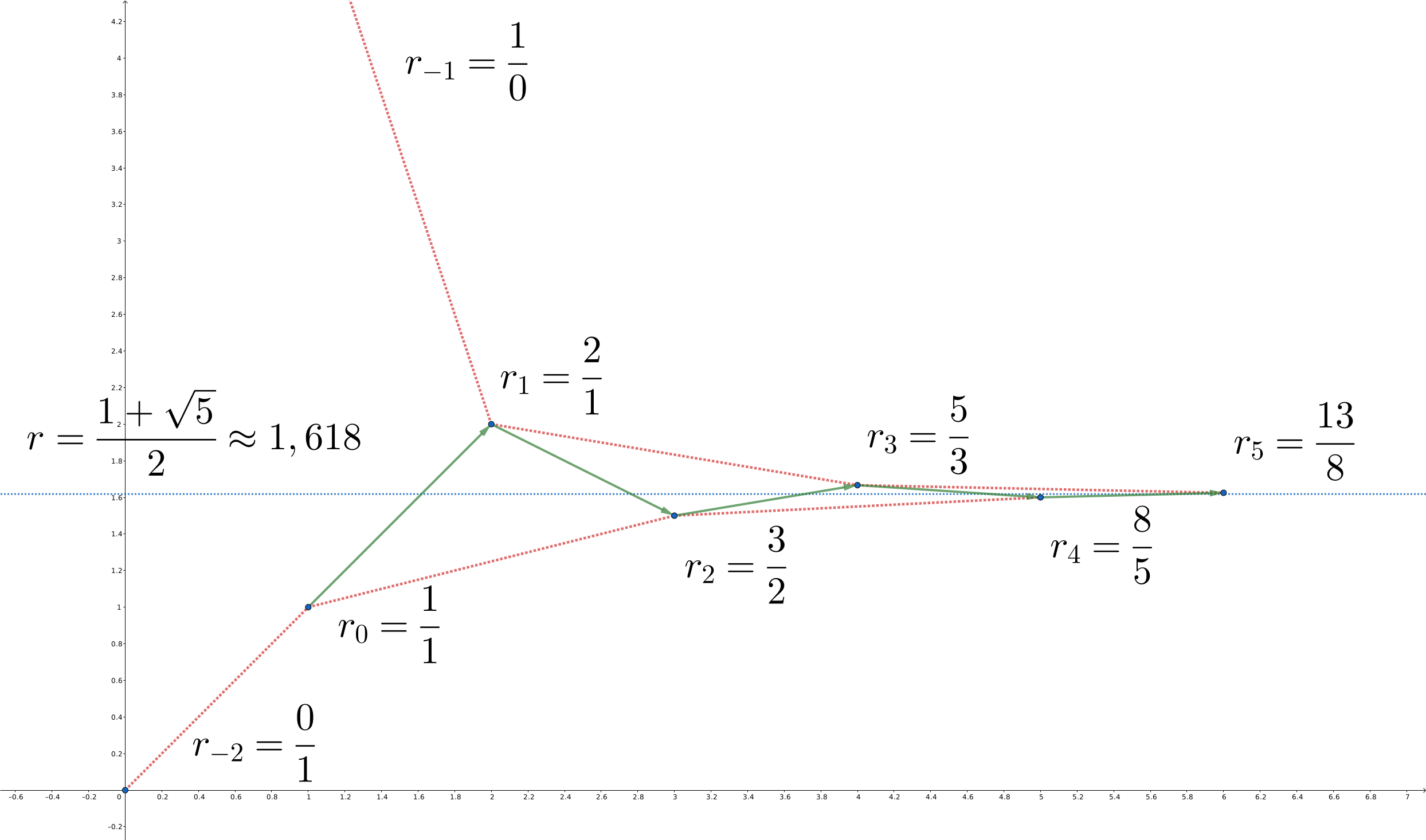
is positive (negative) when is even (odd). At the same time, because the recurrence holds, the denominator grows at least as fast as the Fibonacci sequence. Thus, the difference between adjacent terms must approach zero. This shows that the even-indexed and odd-indexed convergents approach the same limit from below and above, respectively. This proves that every infinite simple continued fraction converges. The way convergents approach the corresponding real number is shown below:
Upper and lower convergents
For a real number and its convergent , if (), then is called an upper (lower) convergent of .
We have already shown that upper convergents are exactly the odd-indexed convergents, while lower convergents are exactly the even-indexed convergents.
Using the difference formula, we can write the real number as an alternating series:
The convergents and remainders in the definition of a continued fraction are the partial sums and remainders of this series.
The difference formula also gives a direct estimate of the error produced when a convergent approximates a real number:
Error
Let be the convergent of the real number with index . Then
Here is the remainder of the real number with index . Consequently,
Proof
Since , and the difference formula for convergents also holds for formal continued fractions, we have
where is the denominator of the -th convergent of this formal continued fraction obtained from the recurrence.
To complete the following inequality estimate, we only need to note that when , we always have
so
Therefore,
To obtain the outer bounds, also note that .
The difference formula in this section has the following simple corollary: all convergents are reduced.
Corollary
For any real number , if the numerator and denominator of the convergent are given by the recurrence, then is a reduced fraction, that is, .
Proof
Apply Bézout's identity to the difference formula.
In fact, solutions to a binary linear Diophantine equation can be found using continued fractions.
Solving a binary linear Diophantine equation
Given , find such that .
Solution
Although this problem is usually solved using the extended Euclidean algorithm, it can also be solved using continued fractions.
Suppose that . We proved above that . Replacing and with and gives
where . If divides , one solution is and ; otherwise, there is no solution.
C++
// Return (x,y) such that Ax+By=C.
// Assume that such (x,y) exists.
auto dio(int A, int B, int C) {
  std::vector<int> p, q;
  std::tie(p, q) = convergents(fraction(A, B));
  C /= A / p.back();
  int t = p.size() % 2 ? -1 : 1;
  return std::make_pair(t * C * q.end()[-2], -t * C * p.end()[-2]);
}
Python
# Return (x, y) such that Ax+By=C.
# Assume that such (x, y) exists.
def dio(A, B, C):
    p, q = convergents(fraction(A, B))
    C //= A // p[-1]  # divide by gcd(A, B)
    t = (-1) if len(p) % 2 else 1
    return t * C * q[-2], -t * C * p[-2]
Diophantine approximation
An important application of continued-fraction theory is Diophantine approximation. Diophantine approximation means approximating real numbers with rational numbers. Of course, because rational numbers are dense, we can obtain approximations with arbitrarily small error if there are no restrictions. Therefore, we need to restrict the rational numbers that may be used, for example, to rational numbers whose denominators are below a given value. This section discusses the relationship between best approximations under such restrictions and continued fractions.
Approximating real numbers with convergents
First, the error estimate for convergents immediately gives the following result:
Theorem (Dirichlet)
For an irrational number , there exist infinitely many reduced fractions such that
holds.
Proof
By the error estimate for convergents, for an irrational number , the convergent with index , satisfies
Checking the proof of the error formula shows that equality cannot hold for any irrational number . Therefore, the numerators and denominators of all its convergents satisfy the requirement.
This theorem can also be viewed as a corollary of the Dirichlet approximation theorem. This is nearly the best possible result. The exponent in the denominator on the right-hand side cannot be improved, but the constant can be improved. Hurwitz's theorem says that the right-hand side can be reduced to , and this is the best possible bound.
Hurwitz's theorem
For an irrational number , there exist infinitely many reduced fractions such that
holds, and the on the right-hand side cannot be replaced by a larger real number.
Proof (Borel)
Borel actually proved that among any three consecutive convergents of an irrational number , at least one necessarily satisfies the condition above. Since there are infinitely many convergents and all are reduced fractions, the first part of Hurwitz's theorem follows.
We argue by contradiction. Suppose that there is an irrational number and three of its convergents such that
hold. Since adjacent convergents must lie on opposite sides of , the difference formula gives
This can be written as an inequality for the quotient :
The left-hand side is rational and the right-hand side is irrational, so equality cannot hold. Since , we obtain
Similarly, we can prove
However, by the recurrence and the two inequalities, we have
This contradicts the definition of a simple continued fraction. Hence Borel's conclusion holds.
To show that this bound is the best possible, it suffices to find an such that for every , only finitely many reduced fractions satisfy
We now prove that is such an .3
Let be the conjugate root of . Both are roots of the equation . Thus, for every real number ,
Substituting the reduced fraction gives
For , we can directly solve for , so there cannot be infinitely many solutions satisfying the inequality above.
The proofs of these theorems show that convergents provide fairly good Diophantine approximations. However, they are not necessarily the best approximations. To discuss best approximations, we need to specify a measure of the quality of an approximation. There are usually two choices.
Best-approximation results may fail in some cases
The next two sections state several results about best approximations. These results may fail for certain uninteresting cases. For example, both definitions of best approximation require a strict inequality, but for a half-integer with , its continued fraction can be written as . In this case, the denominators of its first two convergents and are both , and their distances from are equal. Thus, neither is a best approximation. In stating the results of this section, the reader should assume that such cases have been excluded. If the reader is not concerned with the last few convergents, or only cares about approximating irrational numbers, these extra complications can be ignored.
First-kind best approximations: intermediate fractions
First-kind best approximations use
to measure the quality of an approximation.
Best approximation of the first kind
For a real number and a rational number , if for every with we have
then the rational number is called a best approximation of the first kind of the real number .
A first-kind best approximation need not be a convergent; it may be a more general fraction.
Intermediate fractions
Suppose that a real number has the convergent , and let the integer satisfy 4. Then the fraction is called an intermediate fraction, semiconvergent, or secondary convergent of .5
As with convergents, an intermediate fraction greater (less) than is called an upper (lower) semiconvergent.
By the recurrence, an intermediate fraction can be written as
It is necessarily a reduced fraction and lies between the convergents and . As increases, it gradually approaches ; taking the case where is even as an example,
Because the numerators and denominators of convergents both increase, the numerator and denominator of an intermediate fraction () lie between those of and . If these fractions are ordered by denominator, the intermediate fractions are some fractions lying between adjacent convergents.
All first-kind best approximations are intermediate fractions, but not every intermediate fraction is a first-kind best approximation.
Theorem
Every first-kind best approximation is an intermediate fraction.
Proof
Since , a first-kind best approximation must lie between and . All intermediate fractions can be ordered from small to large as
Intermediate fractions of the same order occur consecutively, and there are no gaps between intermediate fractions of different orders. This means that any rational number lying between and , namely must lie between two intermediate fractions and of the same order. Suppose without loss of generality that it is not an intermediate fraction and is smaller than , so
On the one hand,
On the other hand,
Therefore,
In other words, the denominator of the rational number is larger than the denominator of , but it is not a better approximation:
Therefore, it cannot be a first-kind best approximation. This shows that a fraction that is not an intermediate fraction cannot be a first-kind best approximation; equivalently, every first-kind best approximation is an intermediate fraction.
Conversely, we cannot assert that every intermediate fraction is a first-kind best approximation. However, we can give the condition under which an intermediate fraction is a first-kind best approximation.
Theorem
Every convergent is a first-kind best approximation. In addition, let . Then the intermediate fraction is a first-kind best approximation if and only if , or and .
Proof
We will show below that every convergent is a second-kind best approximation, and hence is necessarily a first-kind best approximation. The key issue is the intermediate fractions that are not convergents.
As stated earlier, the denominator of an intermediate fraction lies between those of and and increases as increases, while gradually approaches and hence gets closer to . For example, when , its relative positions with the neighboring intermediate fractions satisfy
Since the denominator of is smaller than that of , the necessary condition for to be a first-kind best approximation is that it, relative to , give a closer approximation to . This is also sufficient: as a convergent, no fraction with a denominator smaller than that of is a closer approximation. An intermediate fraction with a denominator larger than that of is necessarily of the same order as and, having a smaller denominator, is necessarily farther from . Direct calculation gives the errors of the convergent and intermediate fraction:
Here we used . Thus, is closer than to and is a first-kind best approximation if and only if
There are three possible cases:
- If , then . Since both sides are integers, , so . In this case, is not a first-kind best approximation;
- If , then . Since both sides are integers, . In this case, is a first-kind best approximation;
- If is even, there is a third case, namely . The condition above is equivalent to , or .
Therefore, if all first-kind best approximations of a real number are ordered by increasing denominator, they split into several segments according to their relation to . Each segment consists of several (possibly zero) consecutive intermediate fractions of the same order and always ends with a convergent. Within a segment they remain on the same side of , while successive segments alternate between the two sides of .
Example: first-kind best approximations of
Since , its first 15 first-kind best approximations in order of increasing denominator are:
Second-kind best approximations
Second-kind best approximations use to measure the quality of an approximation.
Best approximation of the second kind
For a real number and a rational number , if for every with we have
then the rational number is called a best approximation of the second kind of the real number .
The condition for a second-kind best approximation is equivalent to
Because , the condition for a second-kind best approximation is stricter than that for a first-kind best approximation.
A second-kind best approximation can be, and only can be, a convergent.
Theorem
Every second-kind best approximation is a convergent, and every convergent is also a second-kind best approximation.
Proof
To prove the first part, since every second-kind best approximation is also a first-kind best approximation, it suffices to show that an intermediate fraction that is not a convergent cannot be a second-kind best approximation. Let be an intermediate fraction but not a convergent. Suppose that ; then
The error between and satisfies
and using the error estimate for convergents, we always have
so the approximation by is no better than the approximation by , whose denominator is smaller. Hence it cannot be a second-kind best approximation.
Conversely, to prove the second part, every convergent is a second-kind best approximation. We need to show that for every fraction with , . Ignoring the half-integer case, we may assume . First, the error estimate for convergents gives
Equality holds throughout if and only if and it is the final term of the continued fraction. Excluding this case, is strictly worse than .
Take any fraction with . Since the difference formula gives , Cramer's rule shows that the linear system
necessarily has a unique integer solution . If , then , a contradiction. Otherwise, , so and have opposite signs. Since and also have opposite signs, and have the same sign, and therefore
The final inequality is strict because is strictly worse than and . This proves that is a second-kind best approximation.
This property shows that convergents really are quite good Diophantine approximations.
Identifying convergents
Second-kind best approximations provide a necessary and sufficient condition for determining whether a fraction is a convergent. This means that we can determine whether a fraction is a convergent by checking its relative approximation quality. Legendre's criterion provides a way to identify convergents from the absolute quality of the approximation. The original statement of Legendre's criterion gives a necessary and sufficient condition, but its form is not practical. This section gives a simplified version of Legendre's criterion and explains that it omits few convergents.
Theorem (Legendre)
For a real number and a fraction , if
then is necessarily a convergent of .
Proof
Let and be constants satisfying
Expand the rational number as a continued fraction . A rational number has two continued-fraction representations whose values differ by exactly one, so we can choose the representation for which , and let the convergent of this representation be . Let the real number satisfy
Then necessarily
Hence,
This shows that
Expand as a continued fraction . Then
This is a valid simple continued fraction, so is a convergent of .
In fact, this proof shows that the necessary and sufficient condition for to be a convergent is in the proof above, which is precisely the original form of Legendre's criterion.
This criterion shows that any approximation that is sufficiently good must be a convergent. The next theorem shows that there are enough convergents of this quality: at least half of the convergents satisfy the condition.
Theorem (Valhen)
Among any two consecutive convergents of a real number , at least one satisfies
Proof
Suppose otherwise. There is a real number with two consecutive convergents and satisfying
Since lies between and ,
This implies . Therefore, necessarily and . The first two convergents are then and . Thus the only counterexample to the statement is a half-integer, which, as explained earlier, is not considered in this article.
Geometric Interpretation
The theory of continued fractions has an elegant geometric interpretation.
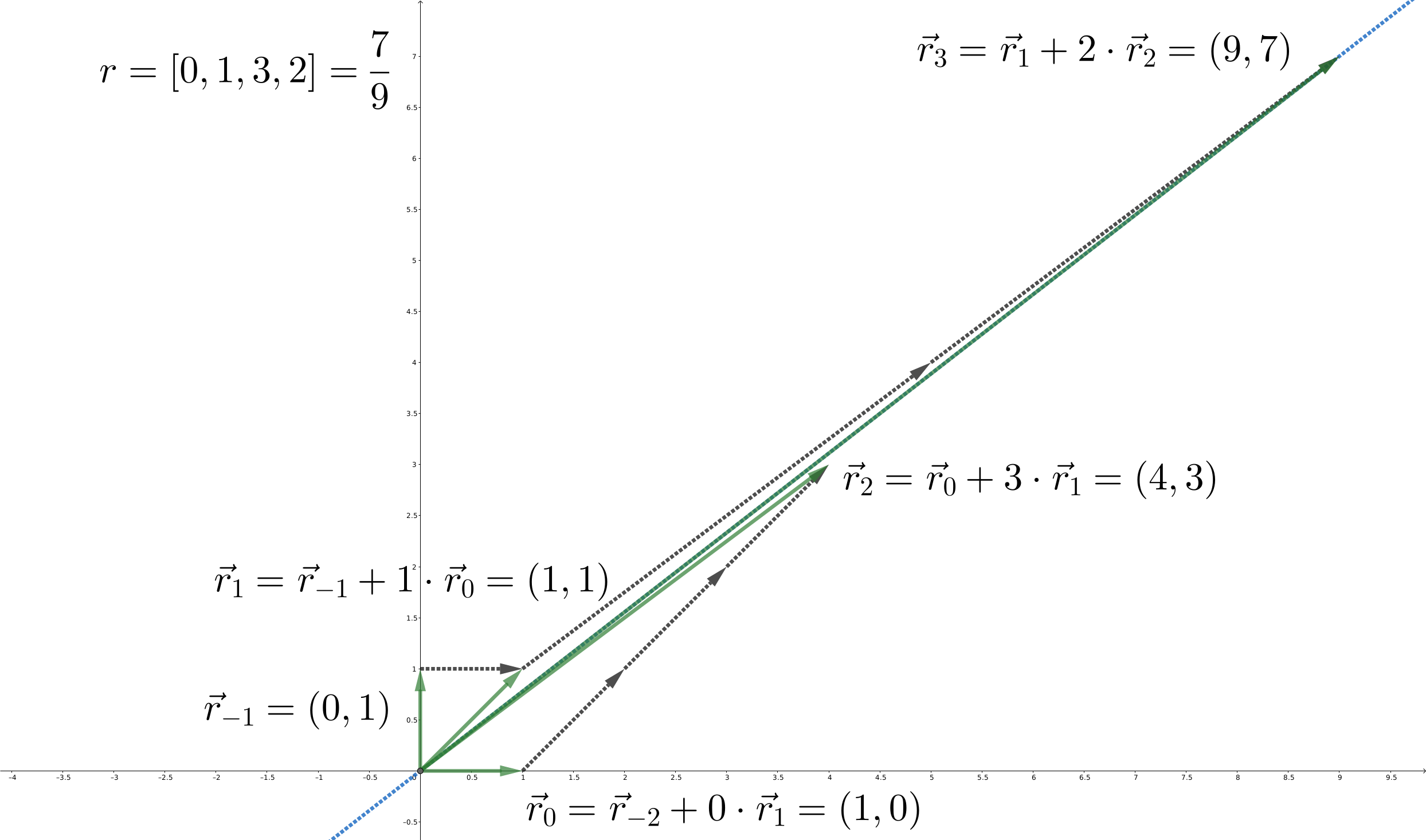
As shown in the figure, for a real number , the line divides the lattice points in the first quadrant (including points on the - and -axes but excluding the origin; this convention applies below) into two parts, above and below. When is rational, points on the line are counted both as points above the line and as points below it. Consider the convex hulls of these two sets of points. Then the odd-indexed convergents are the vertices of the convex hull of the upper part, and the even-indexed convergents are the vertices of the convex hull of the lower part. The lattice points on the line segment between two adjacent vertices of a convex hull are the intermediate fractions. The figure shows the convergents and intermediate fractions (gray points) for .
Most of the conclusions about continued fractions above have corresponding geometric interpretations:
Geometric Interpretation
-
Each fraction corresponds to a lattice point in the first quadrant; the magnitude of the fraction corresponds to the slope of the line joining the point to the origin.
-
The direction vector of the line is . Using the concept of the cross product , the sign of determines whether a point lies above or below the line. Thus, points above the line correspond to fractions greater than or equal to , while points below the line correspond to fractions less than or equal to . The absolute value of the cross product, , is proportional to the distance from to the line :
which corresponds to how closely the fraction approximates the real number .
-
If the point corresponding to the convergent is denoted by , then the recurrence can be written as
The starting points of the recurrence are and .
-
For an integer , if , then the point
lies on the segment joining and . These points correspond to the intermediate fractions .
-
All convergents and intermediate fractions can be constructed geometrically. Start with the points and . The two points lie on opposite sides of the line , which means that and have opposite signs. Add to by vector addition until it is no longer possible to continue without crossing the line ; call the result . It is still on the opposite side from . Then add to until it is no longer possible to continue without crossing the line ; call the result . It is still on the opposite side from . This process can continue indefinitely, unless some lands exactly on the line after finitely many steps. The latter means that and are collinear, that is, is rational. This process produces the figure shown above. Boris Delaunay vividly called it the nose-streching algorithm6.
-
To quickly calculate how many times needs to be added to at each step, we can use the cross product. Since and have opposite signs, let denote the result of adding to times. Then does not change sign exactly when the line has not been crossed. Before the sign changes, the absolute value of gradually decreases. Define
Then the maximum number of decreases is
This is the -th term of the continued-fraction expansion. Moreover, is the remainder of the continued-fraction expansion and satisfies
This is the continued-fraction relation .
-
Since each vector addition changes by a step of size , the final remaining distance must be strictly smaller than . This shows that the approximation quality of the convergents, measured by , strictly improves as increases.
-
Using the rules of the cross product,
By induction,
This is the difference formula for convergents, .
-
The area between the upper and lower convex hulls can be partitioned into several (possibly infinitely many) triangles, each with vertices , , and . The area of such a triangle is
By Pick's theorem, if and are respectively the numbers of lattice points in the interior and on the boundary of the triangle, then
It is also known that the triangle boundary already contains the lattice points . Therefore, it must have and . Thus, there are no more lattice points on the edges of the triangle and none in its interior. In other words, and are coprime, the intermediate fractions are all the lattice points on the edge joining and , and every lattice point in the first quadrant lies inside one of the two convex hulls.
The upper and lower convex hulls obtained in this way are called the Klein polygon. Similar definitions can be made in higher-dimensional spaces, yielding the Klein polyhedron, which generalizes the concept of continued fractions to higher-dimensional spaces.
The Continued-Fraction Tree
Main article: Stern–Brocot tree and Farey sequence
The Stern–Brocot tree is a binary search tree storing all fractions in . A finite continued fraction actually encodes the path from the root to the position of a fraction in the Stern–Brocot tree. In other words, the continued-fraction representation of a rational number means that, starting from the tree root , we first move to the right child times, then to the left child times, alternating directions, until moving times in one direction. Note that only the continued-fraction representation ending in may be used here.
Interpreting a continued-fraction representation as a path in the Stern–Brocot tree gives an algorithm for comparing continued fractions.
Comparing Continued-Fraction Values
Given continued fractions and , compare their values.
Solution
First convert both continued-fraction representations to forms ending in . Without loss of generality, assume that the representations given in the problem already have this form, so . Since even positions (with indices starting from ) give the number of moves to the right and odd positions give the number of moves to the left, if and only if, in lexicographic order,
Compared with the continued-fraction representations, alternately add positive and negative signs, remove the final , and pad shorter positions with .
C++
// Expand [..., n] to [..., n-1, 1] if needed.
void expand(std::vector<int>& a) {
  if (a.size() == 1 || a.back() > 1) {
    --a.back();
    a.push_back(1);
  }
}

// Check if a is smaller than b.
bool less_than(std::vector<int> a, std::vector<int> b) {
  expand(a);
  expand(b);
  for (int i = 0; i < a.size() - 1 || i < b.size() - 1; ++i) {
    int d = (i < a.size() - 1 ? a[i] : 0) - (i < b.size() - 1 ? b[i] : 0);
    if (i & 1) d = -d;
    if (d < 0) {
      return true;
    } else if (d > 0) {
      return false;
    }
  }
  return false;
}
Python
# Expand [..., n] to [..., n-1, 1] if needed.
def expand(a):
    if a[-1] != 1 or len(a) == 1:
        a[-1] -= 1
        a.append(1)
    return a


# Check if a is smaller than b.
def less_than(a, b):
    a = expand(a)
    b = expand(b)
    a = [(-1) ** i * a[i] for i in range(len(a))]
    b = [(-1) ** i * b[i] for i in range(len(b))]
    return a < b
Best Interior Point
Given , find the rational number such that and is minimal.
Solution
Since the Stern–Brocot tree is both a binary search tree for fractions in and a Cartesian tree of pairs , the problem can almost be transformed into finding the LCA (lowest common ancestor) of two nodes in the Stern–Brocot tree. However, an LCA only handles the closed-interval case, where the LCA may itself be an endpoint. To avoid additional case analysis, we can first construct and , and then compute their LCA. Once the paths from the root to the nodes have been computed using continued fractions, the LCA is simply their longest common path.
To construct , first move right (left) once at node , and then move left (right) times. In the language of continued fractions, for a fraction , we know that must be and , respectively. Thus, we only need to compare these two continued fractions and define the larger (smaller) one as .
C++
// Get X +- EPSILON.
auto pm_eps(std::vector<int> a) {
  constexpr int inf = 0x3f3f3f3f;
  // Deal with empty continued fraction for 1/0.
  if (a.empty()) {
    a.emplace_back(inf);
  }
  auto b = a;
  expand(b);
  a.emplace_back(inf);
  b.emplace_back(inf);
  return less_than(a, b) ? std::make_pair(a, b) : std::make_pair(b, a);
}

// Find the lexicographically smallest (q, p)
//   such that p0/q0 < p/q < p1/q1.
auto middle(int p0, int q0, int p1, int q1) {
  auto a0 = pm_eps(fraction(p0, q0)).second;
  auto a1 = pm_eps(fraction(p1, q1)).first;
  std::vector<int> a;
  for (int i = 0; i < a0.size() || i < a1.size(); ++i) {
    if (a0[i] == a1[i]) {
      a.emplace_back(a0[i]);
    } else {
      a.emplace_back(std::min(a0[i], a1[i]) + 1);
      break;
    }
  }
  auto pq = convergents(a);
  return std::make_pair(pq.first.back(), pq.second.back());
}
Python
# Get X +- EPSILON.
def pm_eps(a):
    # Deal with empty continued fraction for 1/0.
    if not a:
        a.append(float("inf"))
    b = expand(a.copy())
    a.append(float("inf"))
    b.append(float("inf"))
    return (a, b) if less_than(a, b) else (b, a)


# Find the lexicographically smallest (q, p)
#   such that p0/q0 < p/q < p1/q1.
def middle(p0, q0, p1, q1):
    a0 = pm_eps(fraction(p0, q0))[1]
    a1 = pm_eps(fraction(p1, q1))[0]
    a = []
    for i in range(min(len(a0), len(a1))):
        if a0[i] == a1[i]:
            a.append(a0[i])
        else:
            a.append(int(min(a0[i], a1[i])) + 1)
            break
    p, q = convergents(a)
    return p[-1], q[-1]
GCJ 2019, Round 2 - New Elements: Part 2
Given pairs of positive integers , find a pair of positive integers such that is strictly increasing. Among all pairs satisfying the requirement, output the lexicographically smallest one.
Solution
Let and without loss of generality. The problem becomes finding such that all are integers. These pairs can be divided into four cases:
- The case can be ignored because we have already assumed ;
- The case directly gives IMPOSSIBLE;
- The case is equivalent to the constraint ;
- The case is equivalent to the constraint .
Therefore, let be the largest among the fourth case, and let be the smallest among the third case. The original problem becomes finding the lexicographically smallest such that .
C++
void solve() {
  int n;
  std::cin >> n;
  std::vector<int> C(n), J(n);
  // p0/q0 < y/x < p1/q1
  int p0 = 0, q0 = 1, p1 = 1, q1 = 0;
  bool fail = false;
  for (int i = 0; i < n; ++i) {
    std::cin >> C[i] >> J[i];
    if (i) {
      int A = C[i] - C[i - 1];
      int B = J[i] - J[i - 1];
      if (A <= 0 && B <= 0) {
        fail = true;
        break;
      } else if (B > 0 && A < 0) {  // y/x > (-A)/B if B > 0
        if ((-A) * q0 > p0 * B) {
          p0 = -A;
          q0 = B;
        }
      } else if (B < 0 && A > 0) {  // y/x < A/(-B) if B < 0
        if (A * q1 < p1 * (-B)) {
          p1 = A;
          q1 = -B;
        }
      }
    }
  }
  if (fail || p0 * q1 >= p1 * q0) {
    printf("IMPOSSIBLE\n");
  } else {
    auto pq = middle(p0, q0, p1, q1);
    printf("%d %d\n", pq.first, pq.second);
  }
}
Python
def solve():
    n = int(input())
    C = [0] * n
    J = [0] * n
    # p0/q0 < y/x < p1/q1
    p0, q0 = 0, 1
    p1, q1 = 1, 0
    fail = False
    for i in range(n):
        C[i], J[i] = map(int, input().split())
        if i > 0:
            A = C[i] - C[i - 1]
            B = J[i] - J[i - 1]
            if A <= 0 and B <= 0:
                fail = True
                break
            elif B > 0 and A < 0:  # y/x > (-A)/B if B > 0
                if (-A) * q0 > p0 * B:
                    p0, q0 = -A, B
            elif B < 0 and A > 0:  # y/x < A/(-B) if B < 0
                if A * q1 < p1 * (-B):
                    p1, q1 = A, -B
    if fail or p0 * q1 >= p1 * q0:
        return "IMPOSSIBLE"
    p, q = middle(p0, q0, p1, q1)
    return str(p) + " " + str(q)
To learn more about the properties and applications of the Stern–Brocot tree, see its main article.
Fractional Linear Transformations
Another important concept related to continued fractions is the fractional linear transformation.
Fractional Linear Transformation
A fractional linear transformation is a function of the form
where and .
About the Condition
It is easy to verify that when , the function may be undefined or constant.
Fractional linear transformations have the following properties:
Properties of Fractional Linear Transformations
Let be fractional linear transformations, and let the matrix formed by the coefficients of be
Then they have the following properties:7
- The composition and inverse transformation of fractional linear transformations are still fractional linear transformations; in other words, all fractional linear transformations form a group;
- A fractional linear transformation is unchanged when all its coefficients are multiplied by the same nonzero constant: for any , if , then ;
- The coefficient matrix of the composition of fractional linear transformations is the product of their coefficient matrices: if , then ;
- The coefficient matrix of the inverse transformation of a fractional linear transformation is the inverse of its coefficient matrix: if , then .
Proof
Here we provide only the forms of the composition and inverse transformation of fractional linear transformations. Once these forms are obtained, all the properties are easy to verify.
The composition of fractional linear transformations and :
The inverse transformation of the fractional linear transformation :
A finite continued fraction can be viewed as the result of composing a sequence of fractional linear transformations. Let
Then the finite continued fraction
Here, the value of a fractional linear transformation at is , the limit of the function as .
For a general continued fraction, let the remainder of the real number be , that is, . Then
This also gives the form of the fractional linear transformation .
The expression can of course also be verified directly. Initially,
Then, if has the form
the composition formula for fractional linear transformations gives
This inductively yields the form above. Fractional linear transformations also provide another perspective for understanding the recurrence formula and initial conditions.
DMOPC '19 Contest 7 P4 - Bob and Continued Fractions
Given a positive-integer array and queries, each query gives and asks for the value of .
Solution
Interpreting a continued fraction as the value at of a composition of fractional linear transformations, we only need to be able to query the composition of a segment of fractional linear transformations many times. Since every fractional linear transformation can be inverted, we can preprocess prefix products and answer queries by taking differences, in time; if updates are needed, structures such as a segment tree can be used for storage.
C++
#include <algorithm>
#include <iostream>
#include <tuple>
#include <vector>

constexpr int M = 1e9 + 7;

// FLTs. Essentially 2x2 matrix.
struct FracLinearTrans {
  int mat[4];

  FracLinearTrans() : mat{} {}

  FracLinearTrans(int x) : mat{x, 1, 1, 0} {}

  FracLinearTrans(int a, int b, int c, int d) : mat{a, b, c, d} {}

  FracLinearTrans operator*(const FracLinearTrans& rhs) const {
    return FracLinearTrans(
        ((long long)mat[0] * rhs.mat[0] + (long long)mat[1] * rhs.mat[2]) % M,
        ((long long)mat[0] * rhs.mat[1] + (long long)mat[1] * rhs.mat[3]) % M,
        ((long long)mat[2] * rhs.mat[0] + (long long)mat[3] * rhs.mat[2]) % M,
        ((long long)mat[2] * rhs.mat[1] + (long long)mat[3] * rhs.mat[3]) % M);
  }

  FracLinearTrans inv() const {
    return FracLinearTrans(mat[3], M - mat[1], M - mat[2], mat[0]);
  }
};

int main() {
  int n, q;
  std::cin >> n >> q;
  // Get prefix sum of FLTs.
  std::vector<FracLinearTrans> ps(1, {1, 0, 0, 1});
  ps.reserve(n + 1);
  for (int i = 1; i <= n; ++i) {
    int a;
    std::cin >> a;
    ps[i] = ps[i - 1] * FracLinearTrans(a);
  }
  // Query.
  for (; q; --q) {
    int l, r;
    std::cin >> l >> r;
    // Difference.
    auto res = ps[l - 1].inv() * ps[r];
    int u = res.mat[0], d = res.mat[2];
    // Correct signs.
    if (!(l & 1)) {
      if (u) u = M - u;
      if (d) d = M - d;
    }
    printf("%d %d\n", u, d);
  }
  return 0;
}
Python
# PYTHON IS TOO SLOW TO PASS THIS PROBLEM.
# JUST FOR REFERENCE.
M = 10**9 + 7


def mul(a, b):
    return (
        (a[0] * b[0] + a[1] * b[2]) % M,
        (a[0] * b[1] + a[1] * b[3]) % M,
        (a[2] * b[0] + a[3] * b[2]) % M,
        (a[2] * b[1] + a[3] * b[3]) % M,
    )


def inv(a):
    return (a[3], M - a[1], M - a[2], a[0])


n, q = map(int, input().split())
ps = [(1, 0, 0, 1)]
# Get presum.
for a in map(int, input().split()):
    ps.append(mul(ps[-1], (a, 1, 1, 0)))
for _ in range(q):
    l, r = map(int, input().split())
    res = mul(inv(ps[l - 1]), ps[r])
    u, d = res[0], res[2]
    if l % 2 == 0:
        if u:
            u = M - u
        if d:
            d = M - d
    print(u, d)
Arithmetic Operations on Continued Fractions
Using fractional linear transformations, we can perform the four arithmetic operations on continued fractions. This algorithm was first proposed by Gosper.
The foundation of the algorithm is computing the fractional linear transformation of a continued fraction. This section uses finite continued fractions as an example, but because producing each output term only requires reading finitely many terms from the input continued fractions, it also applies to infinite continued fractions and can compute to arbitrary precision. Combined with the continued-fraction comparison algorithm above, it can exactly compare differences between real numbers to arbitrary precision.
Fractional Linear Transformation of a Continued Fraction
Given a fractional linear transformation and a continued fraction , find the continued-fraction representation of .
Solution
The basic idea is to determine the values of one by one. Define
Since
we can compute the value of by successively composing with . However, if we want the continued-fraction representation of , we do not need to compute the complete value of and then find its continued-fraction representation. We can determine the values of while composing the .
For example, suppose that we have currently computed
and have the same sign. Then is monotone on , and its value must lie between and . Therefore, if
we can determine that this is the integer part of . Composing on the left then gives
We can then continue adding to determine the new integer part, namely . Continuing in this way determines all the values .
The algorithm requires and to have the same sign to ensure that the discontinuity of the function does not lie in . This is always possible because the definition of a simple continued fraction requires all coefficients other than to be positive integers. It follows that and must have the same sign after finitely many steps, and will continue to do so thereafter.
In an implementation, we only need to maintain the coefficient matrix of the current fractional linear transformation and check whether and have the same sign and whether and have the same integer part. Right-composing with gives . If the two integer parts are both , append to the continued fraction of the result and left-compose with ; this is equivalent to computing .
The fractional linear transformation of a continued fraction can already be used to compute arithmetic operations between fractions and continued fractions:
Arithmetic operations between general continued fractions require a bi-fractional linear transformation:
Bi-Fractional Linear Transformation of Continued Fractions
Given a bi-fractional linear transformation and continued fractions and , find the continued-fraction representation of .
Solution
As in the single-variable fractional linear transformation case, to determine the integer part we only need to ensure that the integer part of the current fractional linear transformation remains unchanged over , that is, all have the same sign and
Right composition is replaced by computing and , which likewise can be represented as a linear transformation of the coefficients. Left composition is exactly the same as in the single-variable case; it only requires taking remainders.
Compared with the single-variable case, the two-variable case must decide whether to compose or first. Since the order of composition does not affect the final result, the order can be chosen freely, for example by composing and alternately. Alternatively, use the heuristic of composing first in the dimension with the larger difference between ratios: if , compose first; otherwise, compose first.
Periodic Continued Fractions
As with repeating decimals, if the coefficients of a continued fraction form a repeating sequence, it is called a periodic continued fraction.
Periodic Continued Fraction
Let be a continued fraction, and suppose there are a natural number and a positive integer such that for every . Then is called a periodic continued fraction. The smallest satisfying this condition is called its least positive period, and the sequence that repeats in the continued fraction is called its period. Using the period, a periodic continued fraction can be written as . If can be chosen to be , that is, , it is called a purely periodic continued fraction; otherwise it is called an eventually periodic continued fraction.
Quadratic Irrationals
A concept closely related to periodic continued fractions is the real quadratic irrational (quadratic irrational), that is, an irrational solution of a quadratic equation with integer coefficients. Every quadratic irrational can be written in the form
where are rational numbers and is a positive square-free integer. Quadratic irrationals mentioned in this article are assumed to be real. The conjugate of means .
Euler's result states that every periodic continued fraction is a quadratic irrational.
Theorem (Euler)
Every number represented by a periodic continued fraction is a quadratic irrational.
Proof
For a general periodic continued fraction , let . Then
where both and are fractional linear transformations. Hence, satisfies
Suppose the fractional linear transformation . Then satisfies
Therefore, every periodic continued fraction is a solution of a quadratic equation with integer coefficients. Since every infinite continued fraction is irrational, periodic continued fractions represent quadratic irrationals.
Lagrange's result shows that the converse also holds, so quadratic irrationals and periodic continued fractions are equivalent.
Theorem (Lagrange)
Every quadratic irrational can be represented as a periodic continued fraction.
Proof
The idea is to prove that the remainders eventually repeat. Suppose the quadratic irrational can be written as
where are integers and . This is always possible. For example, any quadratic irrational can be written as
Then set , , and .
The advantage of writing it in this form is that all its remainders can be shown to have a similar form:
where are integers and . The condition ensures that the coefficient before in the numerator of every remainder is .
We can obtain the form of the remainders by mathematical induction. The case is clear. Assume that the form of has been obtained, and let . Then
Suppose also has the analogous form, and substitute it together with into the equation above:
Since the representation of a quadratic irrational as is unique, comparing the coefficients on both sides gives
Substituting the second equation into the first lets us solve for :
Substituting into the second equation then gives :
By the induction hypothesis, , so and are indeed integers, meaning that also has the required form.
Finally, we prove that the remainders can take only finitely many values and therefore must repeat. We obtained earlier that
and for an irrational number, we always have . Its conjugate is
For sufficiently large , this must be less than , because
This shows that
Therefore, can take only finitely many values. Consequently,
Therefore, can also take only finitely many values. Consequently, the remainder has only finitely many possible values, so some value must repeat within infinitely many terms.
The proof of the theorem also gives a recurrence for computing the remainders of a quadratic irrational:
Recurrence for the remainders of a quadratic irrational
Every quadratic irrational can be written in the form
where . For its remainder
are integers satisfying the recurrence
This recurrence can be used directly to compute the continued fraction of a quadratic irrational. According to the proof of the theorem, and . The algorithm's complexity depends on the length of the period, which can be shown to be 8.
Quadratic irrational
Given a quadratic irrational , find its continued-fraction representation. Here and is not a perfect square.
Solution
First rewrite the quadratic irrational in the form above, and then compute it using the recurrence. The terms of the continued fraction are given by . To find the period, store the index at which each pair first appears.
C++
// Return the continued fraction and minimal positive period
//   of a quadratic irrational (x + y * sqrt(n)) / z.
auto quadratic_irrational(int x, int y, int z, int n) {
  int p = x * z;
  int d = n * y * y * z * z;
  int q = z * z;
  int dd = (int)sqrt(n) * y * z;
  int i = 0;
  std::vector<int> a;
  std::unordered_map<size_t, int> used;
  while (!used.count(((1LL << 32) * p) | q)) {
    a.emplace_back((p + dd) / q);
    used[((1LL << 32) * p) | q] = i++;
    p = a.back() * q - p;
    q = (d - p * p) / q;
  }
  return std::make_pair(a, i - used[((1LL << 32) * p) | q]);
}
Python
# Return the continued fraction and minimal positive period
#   of a quadratic irrational (x + y * sqrt(n)) / z.
def quadratic_irrational(x, y, z, n):
    p = x * z
    d = n * y * y * z * z
    q = z * z
    dd = floor(sqrt(n)) * y * z
    i = 0
    a = []
    used = dict()
    while (p, q) not in used:
        a.append((p + dd) // q)
        used[p, q] = i
        p = a[-1] * q - p
        q = (d - p * p) // q
        i += 1
    return a, i - used[p, q]
Tavrida NU Akai Contest - Continued Fraction
Given and , where is not a perfect square and , find the -th convergent of .
Solution
First use the algorithm above to find the period of . Expressing the period as a fractional linear transformation allows us to obtain using binary exponentiation. The parts before the period and the part shorter than one full period must of course be handled separately.
C++
#include <algorithm>
#include <cmath>
#include <iostream>
#include <tuple>
#include <unordered_map>
#include <vector>

// Return the continued fraction and minimal positive period
//   of a quadratic irrational (x + y * sqrt(n)) / z.
auto quadratic_irrational(int x, int y, int z, int n) {
  int p = x * z;
  int d = n * y * y * z * z;
  int q = z * z;
  int dd = (int)sqrt(n) * y * z;
  int i = 0;
  std::vector<int> a;
  std::unordered_map<size_t, int> used;
  while (!used.count(((1LL << 32) * p) | q)) {
    a.emplace_back((p + dd) / q);
    used[((1LL << 32) * p) | q] = i++;
    p = a.back() * q - p;
    q = (d - p * p) / q;
  }
  return std::make_pair(a, i - used[((1LL << 32) * p) | q]);
}

// Fractional Linear Transformation.
struct FracLinearTrans {
  static constexpr int M = 1e9 + 7;
  int mat[4];

  FracLinearTrans(int a, int b, int c, int d) : mat{a, b, c, d} {}

  FracLinearTrans operator*(const FracLinearTrans& rhs) const {
    return FracLinearTrans(
        ((long long)mat[0] * rhs.mat[0] + (long long)mat[1] * rhs.mat[2]) % M,
        ((long long)mat[0] * rhs.mat[1] + (long long)mat[1] * rhs.mat[3]) % M,
        ((long long)mat[2] * rhs.mat[0] + (long long)mat[3] * rhs.mat[2]) % M,
        ((long long)mat[2] * rhs.mat[1] + (long long)mat[3] * rhs.mat[3]) % M);
  }
};

int main() {
  int x, k, L;
  std::cin >> x >> k;
  std::vector<int> a;
  std::tie(a, L) =
      quadratic_irrational(0, 1, 1, x);  // L==a.size()-1 for sqrt(x)
  FracLinearTrans cyc(1, 0, 0, 1);
  for (int i = a.size() - 1; i; --i) {
    cyc = FracLinearTrans(a[i], 1, 1, 0) * cyc;
  }
  // 1/0=Inf.
  FracLinearTrans res(0, 1, 0, 0);
  // Tail terms.
  for (int i = k % L; i; --i) {
    res = FracLinearTrans(a[i], 1, 1, 0) * res;
  }
  // Binary exponentiation.
  for (int b = k / L; b; b >>= 1) {
    if (b & 1) res = cyc * res;
    cyc = cyc * cyc;
  }
  // First term.
  res = FracLinearTrans(a[0], 1, 1, 0) * res;
  printf("%d/%d", res.mat[1], res.mat[3]);
  return 0;
}
Python
from math import sqrt, floor


# Return the continued fraction and minimal positive period
#   of a quadratic irrational (x + y * sqrt(n)) / z.
def quadratic_irrational(x, y, z, n):
    p = x * z
    d = n * y * y * z * z
    q = z * z
    dd = floor(sqrt(n)) * y * z
    i = 0
    a = []
    used = dict()
    while (p, q) not in used:
        a.append((p + dd) // q)
        used[p, q] = i
        p = a[-1] * q - p
        q = (d - p * p) // q
        i += 1
    return a, i - used[p, q]


# Compose (A[0]*x + A[1]) / (A[2]*x + A[3]) and (B[0]*x + B[1]) / (B[2]*x + B[3])
def combine(A, B):
    return [
        t % mod
        for t in [
            A[0] * B[0] + A[1] * B[2],
            A[0] * B[1] + A[1] * B[3],
            A[2] * B[0] + A[3] * B[2],
            A[2] * B[1] + A[3] * B[3],
        ]
    ]


# Binary exponentiation.
def bpow(A, n):
    return (
        [1, 0, 0, 1]
        if not n
        else combine(A, bpow(A, n - 1))
        if n % 2
        else bpow(combine(A, A), n // 2)
    )


mod = 10**9 + 7
x, k = map(int, input().split())
a, T = quadratic_irrational(0, 1, 1, x)

A = (1, 0, 0, 1)  # (x + 0) / (0*x + 1) = x

# apply ak + 1/x = (ak*x+1)/(1x+0) to (Ax + B) / (Cx + D)
for i in reversed(range(1, len(a))):
    A = combine([a[i], 1, 1, 0], A)

C = (0, 1, 0, 0)  # = 1 / 0
while k % T:
    i = k % T
    C = combine([a[i], 1, 1, 0], C)
    k -= 1

C = combine(bpow(A, k // T), C)
C = combine((a[0], 1, 1, 0), C)
print(str(C[1]) + "/" + str(C[3]))
Purely periodic continued fractions
A quadratic irrational has a periodic continued-fraction representation if and only if it is a quadratic irrational; this section gives the necessary and sufficient condition for a real number to have a purely periodic continued-fraction representation.
First, because a purely periodic continued fraction has a form similar to that of a finite continued fraction, we can perform a “reversal” operation. As with the reversal theorem, the continued-fraction representation obtained this way has a definite relationship with the original representation.
Theorem (Galois)
For the purely periodic continued fraction
define
Then and are “reciprocal negative conjugates” of each other; that is, is the negative reciprocal of the conjugate of .
Proof
Since is not required to be the minimal positive period, we may assume without loss of generality that . By the reversal theorem,
Since both sides of each equality are reduced fractions,
For the purely periodic continued fraction , its -st remainder is itself. Therefore,
Thus it satisfies the quadratic equation
Similarly, satisfies
Using the relationships among the coefficients, this equation can be written as
Let . Then and satisfy the same equation. However, , so they are not the same root; they are conjugates of each other, proving the proposition.
Using this observation, Galois further gave a necessary and sufficient condition for a quadratic irrational to have a purely periodic continued-fraction representation.
Theorem (Galois)
A quadratic irrational can be represented as a purely periodic continued fraction if and only if and its conjugate satisfies .
Proof
If is a purely periodic continued fraction, then using the notation above, , so . Its reciprocal negative conjugate is also a continued fraction, so its conjugate satisfies , or equivalently . This proves that every purely periodic continued fraction satisfies the condition.
Conversely, suppose that the quadratic irrational satisfies . For the remainders of , we have
Both sides are quadratic irrationals, so taking conjugates gives
Using this recurrence, we can prove that holds for every .
For , we have , which is clear. For , the definition of a simple continued fraction and imply that . Therefore, assuming , we obtain
This proves inductively that holds for every . Hence,
Since every quadratic irrational has a periodic continued fraction, there is a positive integer and some sufficiently large such that . But then necessarily
Consequently,
This means that the smallest for which holds must be . In other words, can be represented as a purely periodic continued fraction.
Galois's theorem reveals the pattern in the continued-fraction representation of pure quadratic surds—quadratic irrationals of the form .
Corollary
For a rational number , if is irrational, then
and for every , .
Proof
For the quadratic irrational , since and , is a purely periodic continued fraction:
According to the theorem above, its reciprocal negative conjugate has the form
Using the basic properties of continued fractions, we obtain
On the other hand, the continued-fraction representation of also gives
Since the continued-fraction representation of an irrational number is unique, comparing the intermediate coefficients shows that for every .
Example: The continued-fraction expansion of
The continued fraction of can be computed as follows (this is only for illustration; programmatic computation should use the recursive algorithm mentioned above):
The remainders are:
According to Galois's conclusion, the periodic parts of the remainders and are exact reversals, so they are reciprocal negative conjugates of each other. If the period length of is odd, the middle term is its own reciprocal negative conjugate; if the period length is even, no such term exists. The discussion in the section on Pell equations will show that the parity of the period length determines whether the equation has a solution.
The continued-fraction expansion of the quadratic irrational is mainly used to solve Pell equations.
Examples
After mastering the basic concepts, we need to study some concrete examples to understand how continued fractions are applied in algorithmic competitions.
Offline convex hull
Given , find the convex hull of the set of lattice points satisfying and .
Solution
For the unbounded set , the upper convex hull is the line itself. However, as shown below, if we also require , the upper convex hull eventually deviates from the line.
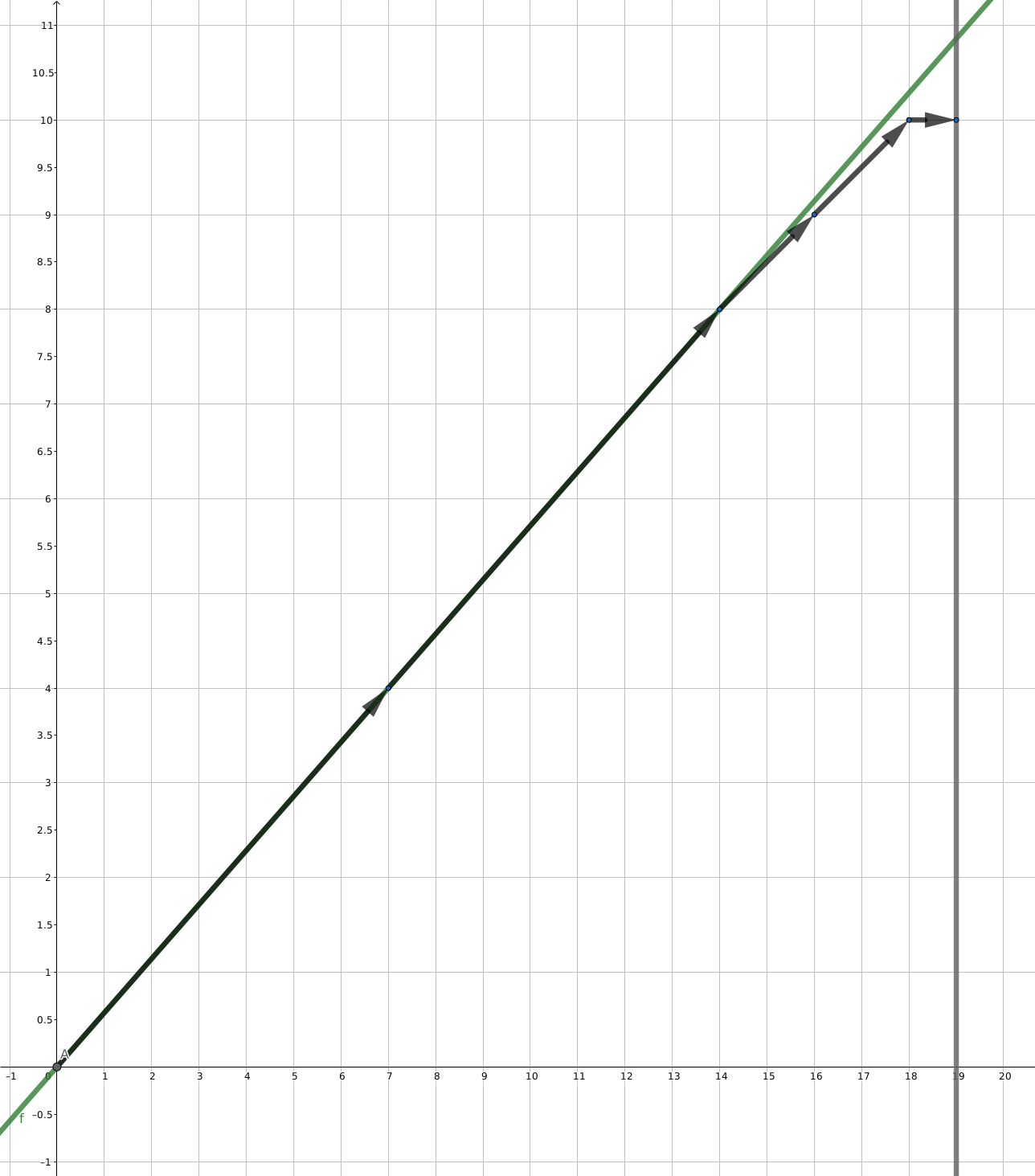
Starting from , we can find all lattice points on the upper convex hull from left to right. Suppose that the last lattice point of the upper convex hull found so far is . We now want to find the next lattice point . The vertex is to the upper right of ; let be their difference. Then necessarily
The second inequality holds because the condition contradicts the fact that is already on the upper convex hull. Looking at the conditions that must satisfy, for different points only the upper bound on changes. Therefore, once this subproblem can be solved, all the lattice points in the original problem can be found recursively.
Let us then consider how to solve the subproblem. Compared with the original problem, the subproblem changes the upper bound of x to and asks for the first lattice point adjacent to the origin on the upper convex hull. Let the solution to the subproblem be . Then and must be coprime (otherwise this would not be the first lattice point), and the slope of the line from the origin is the largest among all lattice points below the line whose -coordinate does not exceed (otherwise it would not lie on the convex hull). According to the geometric interpretation above, such a point must correspond to a lower intermediate convergent of . Since a lower intermediate convergent with a larger denominator is closer to , the subproblem's solution corresponds to the lower intermediate convergent with the largest denominator among all lower intermediate convergents whose denominators do not exceed .
In an actual solution, there is no need to recompute this lower intermediate convergent for every subproblem. We should first compute all convergents, which provides a way to traverse all lower intermediate convergents. Then traverse the lower intermediate convergents in decreasing order of denominator, trying each time to add it to the previous lattice point , and continue until it can no longer be added before trying the next lower intermediate convergent.
There are several obvious optimizations. First, for a lower intermediate convergent , there must be an odd and such that . It is enough to find the largest satisfying , namely . There is no need to worry about going out of range, because the larger lower convergent has already been added. Each time the number of additions is determined, we can directly compute instead of trying them one by one.
The optimized algorithm has complexity . Although a lower intermediate convergent may correspond to many lattice points, not many of them actually become increments. We now show that among all lower intermediate convergents with , at most two increments can occur. Suppose that an increment does occur among these lower intermediate convergents. Then necessarily . Set . If , then the increment has , so after adding the increment we have , and no new increment can occur among these lower intermediate convergents. If , then after adding the increment we necessarily have ; even if another increment occurs in the same interval of lower intermediate convergents, the next one can only have . Thus, at most two increments can occur in such an interval of lower intermediate convergents. This proves that the total time complexity is .
C++
// Find [ah, ph, qh] such that points r[i]=(ph[i], qh[i]) constitute
// upper convex hull of lattice points on 0 <= x <= N and 0 <= y <= r * x,
// where r = [a0, a1, a2, ...] and there are ah[i]-1 integer points on the
// segment between r[i] and r[i+1].
auto hull(std::vector<int> a, int N) {
  std::vector<int> p, q;
  std::tie(p, q) = convergents(a);
  int t = N / q.back();
  std::vector<int> ah = {t};
  std::vector<int> ph = {0, t * p.back()};
  std::vector<int> qh = {0, t * q.back()};

  for (int i = q.size() - 1; i; --i) {
    if (i % 2) {
      while (qh.back() + q[i - 1] <= N) {
        t = (N - qh.back() - q[i - 1]) / q[i];
        int dp = p[i - 1] + t * p[i];
        int dq = q[i - 1] + t * q[i];
        int k = (N - qh.back()) / dq;
        ah.push_back(k);
        ph.push_back(ph.back() + k * dp);
        qh.push_back(qh.back() + k * dq);
      }
    }
  }
  return make_tuple(ah, ph, qh);
}
Python
# Find [ah, ph, qh] such that points r[i]=(ph[i], qh[i]) constitute
# upper convex hull of lattice points on 0 <= x <= N and 0 <= y <= r * x,
# where r = [a0, a1, a2, ...] and there are ah[i]-1 integer points on the
# segment between r[i] and r[i+1].
def hull(a, N):
    p, q = convergents(a)
    t = N // q[-1]
    ah = [t]
    ph = [0, t * p[-1]]
    qh = [0, t * q[-1]]
    for i in reversed(range(len(q))):
        if i % 2 == 1:
            while qh[-1] + q[i - 1] <= N:
                t = (N - qh[-1] - q[i - 1]) // q[i]
                dp = p[i - 1] + t * p[i]
                dq = q[i - 1] + t * q[i]
                k = (N - qh[-1]) // dq
                ah.append(k)
                ph.append(ph[-1] + k * dp)
                qh.append(qh[-1] + k * dq)
    return ah, ph, qh
Timus - Crime and Punishment
Given positive integers , find such that and is as large as possible.
Solution
This problem has an solution: assume without loss of generality that . Since , it is enough to search over . This is sufficient to pass the problem. However, using continued fractions reduces the time complexity to .
For convenience, first change the sign of by the substitution . Let and . The original problem becomes finding the optimal under and , maximizing . For each fixed , the optimal value of is .
Next, we explain why this problem has a solution similar to that of the previous example. Unlike the previous example, which uses lower intermediate convergents to deviate from a line, this problem needs upper intermediate convergents to approach a line. Specifically, is proportional to the distance between and the line . Maximizing is equivalent to minimizing this distance. The goal of the algorithm is to find the feasible lattice point below the line that is closest to it. The idea is to start from the leftmost point and search along the upper convex hull of these lattice points, progressively reducing the distance to the line until the optimum is found.
In the coordinate system, the algorithm starts at and recursively finds and adds the optimal increment , ensuring that the new point is closer to the line than the previous point, without crossing to the other side of the line or making its x-coordinate exceed . If the point already obtained is , then the increment must satisfy
0 $$ Following the idea of searching along a lower convex hull, we only need to find the point with the smallest $\Delta x$ among the points satisfying these conditions. Rewrite the first inequality as\Delta y \le \dfrac{A}{B}\Delta x+\dfrac{C-(By-Ax)}{B}.
According to the [geometric interpretation](#几何解释) above, as long as the constant term on the right is less than $1$, the feasible lattice point $(\Delta x,\Delta y)$ with the smallest x-coordinate must correspond to an upper intermediate convergent. This is because, among all fractions with denominator no larger than its denominator, it is the one that best approaches a real number from above, which can only be an upper intermediate convergent. Each time an increment is added, the upper bound on $\Delta y$ becomes tighter, so intermediate convergents with larger denominators must be examined. Following the idea of the previous example, examine all upper intermediate convergents in increasing order of denominator. If an upper intermediate convergent has neither coordinate out of bounds, add it and update the corresponding upper bound. Once all feasible upper intermediate convergents have been added, the result is the optimum. Compared with the previous problem, this one must ensure that both coordinates remain within bounds, which requires extra care. Using an argument similar to that for the previous example, but replacing the previous $\Delta x$ with $B\Delta y-A\Delta x$, we can show that the complexity of this algorithm is $O(\log\min\{A,B\})$. **C++** ```py // Find (x, y) such that y = (A*x+B)/C, // such that Cy - Ax is max and 0 <= x <= N. auto closest(int A, int B, int C, int N) { // y <= (A*x + B)/C <=> diff(x, y) <= B auto diff = [&](int x, int y) -> int { return C * y - A * x; }; std::vector<int> p, q; std::tie(p, q) = convergents(fraction(A, C)); int qh = 0, ph = B / C; for (int i = 2; i < q.size() - 1; ++i) { if (i % 2 == 0) { while (diff(qh + q[i + 1], ph + p[i + 1]) <= B) { int t = 1 + (diff(qh + q[i - 1], ph + p[i - 1]) - B - 1) / (-diff(q[i], p[i])); int dp = p[i - 1] + t * p[i]; int dq = q[i - 1] + t * q[i]; int k = (N - qh) / dq; if (k == 0) { return std::make_pair(qh, ph); } if (diff(dq, dp) != 0) { k = std::min(k, (B - diff(qh, ph)) / diff(dq, dp)); } qh += k * dq; ph += k * dp; } } } return std::make_pair(qh, ph); } auto solve(int A, int B, int N) { int x, y; std::tie(x, y) = closest(A, N % A, B, N / A); return std::make_pair(N / A - x, y); } ``` **Python** ```py # Find (x, y) such that y = (A*x+B) // C, # such that Cy - Ax is max and 0 <= x <= N. def closest(A, B, C, N): # y <= (A*x + B)/C <=> diff(x, y) <= B def diff(x, y): return C * y - A * x p, q = convergents(fraction(A, C)) qh, ph = 0, B // C for i in range(2, len(q) - 1): if i % 2 == 0: while diff(qh + q[i + 1], ph + p[i + 1]) <= B: t = 1 + (diff(qh + q[i - 1], ph + p[i - 1]) - B - 1) // ( -diff(q[i], p[i]) ) dp = p[i - 1] + t * p[i] dq = q[i - 1] + t * q[i] k = (N - qh) // dq if k == 0: return qh, ph if diff(dq, dp) != 0: k = min(k, (B - diff(qh, ph)) // diff(dq, dp)) qh, ph = qh + k * dq, ph + k * dp return qh, ph def solve(A, B, N): x, y = closest(A, N % A, B, N // A) return N // A - x, y ```June Challenge 2017 - Euler Sum
Find the value of , where is the base of the natural logarithm.
Hint: .9
Solution
This sum equals the number of lattice points in the set . After constructing the convex hull of the lattice points below the line , the Pick theorem can be used to count the lattice points. The time complexity is .
The original problem requires . The C++ code below is only illustrative and does not implement an arbitrary-precision arithmetic class.
C++
// Find sum of floor(k * x) for k in [1, N] and x = [a0; a1, a2, ...]
int sum_floor(std::vector<int> a, int N) {
  N++;
  std::vector<int> ah, ph, qh;
  std::tie(ah, ph, qh) = hull(a, N);

  // The number of lattice points within a vertical right trapezoid
  // on points (0; 0) - (0; y1) - (dx; y2) - (dx; 0) that has
  // a+1 integer points on the segment (0; y1) - (dx; y2).
  auto picks = [](int y1, int y2, int dx, int a) -> int {
    int b = y1 + y2 + a + dx;
    int A = (y1 + y2) * dx;
    return (A + b) / 2 - y2;  // = (A - b + 2) // 2 + b - (y2 + 1)
  };

  int ans = 0;
  for (size_t i = 1; i < qh.size(); i++) {
    ans += picks(ph[i - 1], ph[i], qh[i] - qh[i - 1], ah[i - 1]);
  }
  return ans - N;
}
Python
# Find sum of floor(k * x) for k in [1, N] and x = [a0; a1, a2, ...].
def sum_floor(a, N):
    N += 1
    ah, ph, qh = hull(a, N)

    # The number of lattice points within a vertical right trapezoid
    # on points (0; 0) - (0; y1) - (dx; y2) - (dx; 0) that has
    # a+1 integer points on the segment (0; y1) - (dx; y2) but with
    # the number of points on the vertical right line excluded.
    def picks(y1, y2, dx, a):
        b = y1 + y2 + a + dx
        A = (y1 + y2) * dx
        return (A + b) // 2 - y2  # = (A - b + 2) // 2 + b - (y2 + 1)

    ans = 0
    for i in range(1, len(qh)):
        ans += picks(ph[i - 1], ph[i], qh[i] - qh[i - 1], ah[i - 1])
    return ans - N
NAIPC 2019 - It's a Mod, Mod, Mod, Mod World
Given positive integers , find the value of .
Solution
Since the sum can be rewritten as
this problem can be reduced to the previous one by replacing with . The time complexity of a single query is .
C++
int solve(int p, int q, int n) {
  return p * n * (n + 1) / 2 - q * sum_floor(fraction(p, q), n);
}
Python
def solve(p, q, N):
    return p * N * (N + 1) // 2 - q * sum_floor(fraction(p, q), N)
Library Checker - Sum of Floor of Linear
Given positive integers , find the value of .
Solution
This is the most complicated problem so far. It can be solved using the Euclidean-like algorithm. Here we give an algorithm based on continued fractions, with time complexity .
We can construct the convex hull of all lattice points below with , and use Pick's theorem to count the lattice points. The case was solved earlier. For the general case, we can proceed in two steps. First, progressively approach the line by adding upper intermediate convergents (the second example), until the closest point on the line is found; then progressively move away from the line by adding lower intermediate convergents (the first example).
C++
// Find convex hull of lattice (x, y) such that C*y <= A*x+B.
auto hull(int A, int B, int C, int N) {
  auto diff = [&](int x, int y) -> int { return C * y - A * x; };
  auto a = fraction(A, C);
  std::vector<int> p, q;
  std::tie(p, q) = convergents(a);
  std::vector<int> ah(0), ph(1, B / C), qh(1, 0);
  auto insert = [&](int dq, int dp) -> void {
    int k = (N - qh.back()) / dq;
    if (diff(dq, dp) > 0) {
      k = std::min((int)k, (B - diff(qh.back(), ph.back())) / diff(dq, dp));
    }
    ah.emplace_back(k);
    qh.emplace_back(qh.back() + k * dq);
    ph.emplace_back(ph.back() + k * dp);
  };
  for (int i = 1; i < q.size() - 1; ++i) {
    if (i % 2 == 0) {
      while (diff(qh.back() + q[i + 1], ph.back() + p[i + 1]) <= B) {
        int t = (B - diff(qh.back() + q[i + 1], ph.back() + p[i + 1])) /
                (-diff(q[i], p[i]));
        int dp = p[i + 1] - t * p[i];
        int dq = q[i + 1] - t * q[i];
        if (dq < 0 || qh.back() + dq > N) break;
        insert(dq, dp);
      }
    }
  }
  insert(q.back(), p.back());
  for (int i = q.size() - 1; i; --i) {
    if (i % 2 == 1) {
      while (qh.back() + q[i - 1] <= N) {
        int t = (N - qh.back() - q[i - 1]) / q[i];
        int dp = p[i - 1] + t * p[i];
        int dq = q[i - 1] + t * q[i];
        insert(dq, dp);
      }
    }
  }
  return std::make_tuple(ah, ph, qh);
}

// Sum of floor (Ax+B)/M from 0 to N-1.
auto solve(int N, int M, int A, int B) {
  std::vector<int> ah, ph, qh;
  std::tie(ah, ph, qh) = hull(A, B, M, N);
  // The number of lattice points within a vertical right trapezoid
  // on points (0; 0) - (0; y1) - (dx; y2) - (dx; 0) that has
  // a+1 integer points on the segment (0; y1) - (dx; y2) but with
  // the number of points on the vertical right line excluded.
  auto picks = [&](int y1, int y2, int dx, int a) -> int {
    int b = y1 + y2 + a + dx;
    int A = (y1 + y2) * dx;
    return (A + b) / 2 - y2;  // = (A - b + 2) // 2 + b - (y2 + 1)
  };
  int ans = 0;
  for (int i = 1; i < qh.size(); ++i) {
    ans += picks(ph[i - 1], ph[i], qh[i] - qh[i - 1], ah[i - 1]);
  }
  return ans - N;
}
Python
# Find convex hull of lattice (x, y) such that C*y <= A*x+B.
def hull(A, B, C, N):
    def diff(x, y):
        return C * y - A * x

    a = fraction(A, C)
    p, q = convergents(a)
    ah = []
    ph = [B // C]
    qh = [0]

    def insert(dq, dp):
        k = (N - qh[-1]) // dq
        if diff(dq, dp) > 0:
            k = min(k, (B - diff(qh[-1], ph[-1])) // diff(dq, dp))
        ah.append(k)
        qh.append(qh[-1] + k * dq)
        ph.append(ph[-1] + k * dp)

    for i in range(1, len(q) - 1):
        if i % 2 == 0:
            while diff(qh[-1] + q[i + 1], ph[-1] + p[i + 1]) <= B:
                t = (B - diff(qh[-1] + q[i + 1], ph[-1] + p[i + 1])) // (
                    -diff(q[i], p[i])
                )
                dp = p[i + 1] - t * p[i]
                dq = q[i + 1] - t * q[i]
                if dq < 0 or qh[-1] + dq > N:
                    break
                insert(dq, dp)

    insert(q[-1], p[-1])

    for i in reversed(range(len(q))):
        if i % 2 == 1:
            while qh[-1] + q[i - 1] <= N:
                t = (N - qh[-1] - q[i - 1]) // q[i]
                dp = p[i - 1] + t * p[i]
                dq = q[i - 1] + t * q[i]
                insert(dq, dp)
    return ah, ph, qh


def solve(N, M, A, B):
    ah, ph, qh = hull(A, B, M, N)

    # The number of lattice points within a vertical right trapezoid
    # on points (0; 0) - (0; y1) - (dx; y2) - (dx; 0) that has
    # a+1 integer points on the segment (0; y1) - (dx; y2) but with
    # the number of points on the vertical right line excluded.
    def picks(y1, y2, dx, a):
        b = y1 + y2 + a + dx
        A = (y1 + y2) * dx
        return (A + b) // 2 - y2  # = (A - b + 2) // 2 + b - (y2 + 1)

    ans = 0
    for i in range(1, len(qh)):
        ans += picks(ph[i - 1], ph[i], qh[i] - qh[i - 1], ah[i - 1])
    return ans - N
OKC 2 - From Modular to Rational
There is an unknown rational number with . For a prime , you may query the value of after reducing it modulo that prime. Determine the values of and in no more than ten queries.
This problem is equivalent to finding, in , the value that minimizes , namely .
Solution
According to the Chinese remainder theorem, querying the results modulo multiple primes is equivalent to querying the result modulo the product of those primes. Therefore, this problem can be regarded as querying the result of taking the fraction modulo a sufficiently large modulus , with the numerator and denominator of the fraction to be determined.
For a given modulus , it need not be the case that the pairs satisfying —namely —are unique. Suppose that both and can make this equation hold. Then it necessarily follows that . From the construction of , we know that is coprime to , so , or equivalently, . If is nonzero, then its absolute value is at least . The problem constrains , which means that this difference should not exceed . Thus, taking guarantees that the resulting is unique.
The problem now reduces to this: given a modulus and a remainder , find, for a bound , positive integer pairs with both values no greater than that bound such that . Once it is known that such a solution is unique, it is enough to find the such that the minimum of is attained at , because in that case there is exactly one whose remainder does not exceed . This is precisely the equivalent formulation mentioned above.
In the plane with coordinates , this amounts to finding, for , the lattice point below and closest to the line , because the remainder is directly proportional to the distance between the lattice point and the line. Combining this with the geometric interpretation given earlier, we see that this lattice point must correspond to one of the lower semiconvergents of the rational fraction . The algorithm has complexity .
C++
// Find Q that minimizes Q*r mod m for 1 <= k <= n < m.
int mod_min(int r, int n, int m) {
  auto a = fraction(r, m);
  std::vector<int> p, q;
  std::tie(p, q) = convergents(a);
  for (int i = 2; i < q.size(); ++i) {
    if (i % 2 == 1 && (i + 1 == q.size() || q[i + 1] > n)) {
      int t = (n - q[i - 1]) / q[i];
      return q[i - 1] + t * q[i];
    }
  }
  return 0;
}
Python
# Find Q that minimizes Q*r mod m for 1 <= k <= n < m.
def mod_min(r, n, m):
    a = fraction(r, m)
    p, q = convergents(a)
    for i in range(2, len(q)):
        if i % 2 == 1 and (i + 1 == len(q) or q[i + 1] > n):
            t = (n - q[i - 1]) // q[i]
            return q[i - 1] + t * q[i]
    return 0
Exercises
- UVa OJ - Continued Fractions
- ProjectEuler+ #64: Odd period square roots
- LibreOJ NOI Round #2 - Going It Alone
- Codeforces Round #184 (Div. 2) - Continued Fractions
- Codeforces Round #201 (Div. 1) - Doodle Jump
- Codeforces Round #325 (Div. 1) - Alice, Bob, Oranges and Apples
- POJ Founder Monthly Contest 2008.03.16 - A Modular Arithmetic Challenge
- 2019 Multi-University Training Contest 5 - fraction
- SnackDown 2019 Elimination Round - Election Bait
- Luogu P5179. Fraction
- Luogu P7739. [NOI2021] Password Box
References and Further Reading
- Hardy, G. H., Wright, E. M., Heath-Brown, R., & Silverman, J. (2008). An Introduction to the Theory of Numbers. Oxford Mathematics.
- Zhu Yaochen and Wang Lianxiang, An Introduction to Diophantine Approximation
- FatFish's blog - An Introduction to Continued Fractions
- Simple continued fraction - Wikipedia
- Periodic continued fraction - Wikipedia
- Gosper's original notes on continued fraction arithmetic algorithms
- Understanding Bill Gosper's continued fraction arithmetic (implemented in Python)
The main content of this page is translated from the blog post Continued fractions under the CC-BY-SA 4.0 license, with modifications.
Footnotes
-
The natural number has only the non-standard representation . ↩
-
The translated term comes from Section 6.7 of Concrete Mathematics, translated by Zhang Mingyao and Zhang Fan. ↩
-
At this point, one cannot assume that the reduced fraction must be a convergent, although Legendre's theorem shows that can indeed only be a convergent. In the case of convergents, this can be proved by starting from the error with which a convergent approximates the real number. ↩
-
Different references may handle differently whether the endpoints are included in the range of here. ↩
-
When , it should be understood as a formal continued fraction, equivalent to truncating the continued fraction at its penultimate term. ↩
-
This is not a technical term. It may have been translated from the Russian literature ЦЕПНЫЕ ДРОБИ, in the section Алгоритм «вытягивания носов». ↩
-
These properties show that the group of all fractional linear transformations is isomorphic to the projective linear group . ↩
-
A proof can be found in the references of the Wikipedia page. ↩
-
A proof of the continued fraction expansion of the base of the natural logarithm, , can be found here. ↩