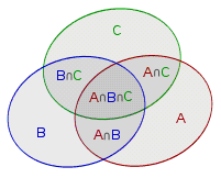
Suppose there are 10 students in a class who like mathematics, 15 who like Chinese, and 21 who like programming. How many students like at least one of these subjects?
Is it 10+15+21=46 students? No, because some students may like both mathematics and Chinese, or Chinese and programming, and some may even like all three.
For convenience, let the sets of students who like Chinese, mathematics, and programming be A,B,C, respectively. Then the total number of students is ∣A∪B∪C∣. As noted above, directly adding the cardinalities ∣A∣,∣B∣,∣C∣ of these three sets counts some elements more than once, so we must subtract ∣A∩B∣,∣B∩C∣,∣C∩A∣. This subtracts a small part too many times, however, so we add it back as ∣A∩B∩C∣. Thus
∣A∪B∪C∣=∣A∣+∣B∣+∣C∣−∣A∩B∣−∣B∩C∣−∣C∩A∣+∣A∩B∩C∣Inclusion–exclusion principle — Venn diagram example
This generalization of the problem is the familiar inclusion–exclusion principle.
Definition
Suppose the elements of U have n different properties, and call the i-th property Pi. The elements having property Pi form the set Si. Then
For each element, use the binomial theorem to calculate how many times it appears. For an element x, suppose it belongs to the sets T1,T2,⋯,Tm. Its number of appearances is
Thus each element appears exactly once, and combining all elements gives the union. QED.
Complements
For the union of sets in a universal set U, we can use inclusion–exclusion. The intersection of sets can instead be obtained by subtracting the union of the complements from the universal set:
i=1⋂nSi=∣U∣−i=1⋃nSi
The right-hand side can be expanded by inclusion–exclusion.
Readers who have encountered inclusion–exclusion are familiar with the material above; what matters more are its applications.
We next give three examples at different levels to demonstrate applications of the inclusion–exclusion principle.
Counting Nonnegative Integer Solutions of an Indeterminate Equation
Counting Nonnegative Integer Solutions of an Indeterminate Equation
Given the equation ∑i=1nxi=m and n constraints xi≤bi, where m,bi∈N. Find the number of nonnegative integer solutions.
Without Constraints
If there is no constraint xi≤bi, the number of nonnegative integer solutions to the equation ∑i=1nxi=m is (n−1m+n−1).
A brief proof uses the stars-and-bars method.
Equivalently, distribute m balls among n boxes, allowing a box to be empty. This cannot be solved directly with a binomial coefficient.
Add n−1 more balls. The problem becomes choosing balls from a sequence of length m+n−1; specifically, choose n−1 balls. These n−1 balls divide the sequence into n parts, which correspond one-to-one to distributions into n boxes. Thus, the number of ways to choose from m+n−1 balls, selecting n−1, is (n−1m+n−1).
Inclusion–Exclusion Model
Let us abstract the model of inclusion–exclusion:
Universal set U: the nonnegative integer solutions of ∑i=1nxi=m
Elements: the variables xi.
Property: the property of xi is the condition satisfied by xi, namely the condition xi≤bi.
The goal is the size of the set in which all variables satisfy their corresponding properties, namely ∣⋂i=1nSi∣.
This can be computed using ∣⋂i=1nSi∣=∣U∣−⋃i=1nSi. The quantity ∣U∣ can be computed with a binomial coefficient, while the latter part is naturally expanded by inclusion–exclusion.
The problem therefore becomes finding the size of an intersection of some Sai. Consider the meaning of Sai: it counts solutions satisfying xai≥bai+1. Their intersection means satisfying all these conditions simultaneously. Thus, in the corresponding indeterminate equation, some variables have lower-bound constraints, while others have none.
Can these lower-bound constraints be removed? We seek nonnegative integer solutions, and some variables have a lower bound greater than 0. We can simply subtract this lower bound, making the lower bound 0, i.e. removing it. Therefore, for
ai<ai+1⋂1≤i≤kSai
the indeterminate equation has the form
i=1∑nxi=m−i=1∑k(bai+1)
This can also be evaluated with a binomial coefficient. The length-ka array is effectively enumerating subsets.
HAOI2008 Coin Shopping
HAOI2008 Coin Shopping
There are four coin denominations; the denomination of the i-th type is Ci. There are n queries. Each query gives the quantity Di of each coin type and a price S, and asks for the number of payment methods.
n≤103,S≤105.
A knapsack solution would have complexity O(4nS), which is too large. The most notable feature is that there are only four coin types. Abstractly, we need the number of nonnegative integer solutions to ∑i=14Cixi=S,xi≤Di.
Using the same inclusion–exclusion method, the property of xi is xi≤Di. Applying the inclusion–exclusion formula, we ultimately need to solve
i=1∑4Cixi=S−i=1∑kCai(Dai+1)
which is an unbounded knapsack problem. It can be precomputed; including the queries, the total complexity is O(4S+24n).
Implementation
#include<iostream>usingnamespace std;
constexprlonglong S = 1e5 + 5;
longlong c[5], d[5], n, s;
longlong f[S];
intmain(){
cin.tie(nullptr)->sync_with_stdio(false);
cin >> c[1] >> c[2] >> c[3] >> c[4] >> n;
f[0] = 1;
for (longlong j = 1; j <= 4; j++)
for (longlong i = 1; i < S; i++)
if (i >= c[j]) f[i] += f[i - c[j]]; // f[i]: number of ways to form price i with the coinsfor (longlong k = 1; k <= n; k++) {
cin >> d[1] >> d[2] >> d[3] >> d[4] >> s;
longlong ans = 0;
for (longlong i = 1; i < 16;
i++) { // Inclusion-exclusion: there are four item types, so iterate from 1 to 2^4-1=15longlong m = s, bit = 0;
for (longlong j = 1; j <= 4; j++) {
if ((i >> (j - 1)) % 2 == 1) {
m -= (d[j] + 1) * c[j];
bit++;
}
}
if (m >= 0) ans += (bit % 2 * 2 - 1) * f[m];
}
cout << f[s] - ans << '\n';
}
return0;
}
Coloring a Complete-Graph Subgraph
The first three examples use inclusion–exclusion directly; this problem requires analyzing it in reverse.
Coloring a Complete-Graph Subgraph
A and B like coloring graphs (not necessarily connected), with the rule that adjacent vertices must receive the same color. Today they play a game on an n-vertex complete graphG=(V,E). They define a scoring function F(S), where S is an edge set and S⊆E. The value of F(S) is the total number of ways to color G′=(V,S) with m colors. Their other rule is that if ∣S∣ is odd, A's score increases by F(S); otherwise B's score increases by F(S). Find the difference between A's and B's scores.
Mathematical Form
The algorithmic direction is not obvious at first glance, so for a difficult problem we first abstract its mathematical form. The score difference is an alternating sum, so powers of -1 can serve as coefficients. We seek
Ans=S⊆E∑(−1)∣S∣−1F(S)
Inclusion–Exclusion Model
We treat the requirement that adjacent vertices have the same color as a property. For now, ignore the coloring rule and color the graph directly with m colors. For the graph G′=(V,S), regard a coloring as an element. The propertyxi=xj means that vertices i and j have the same color (there need not be an edge between i and j).
Define the set corresponding to property xi=xj as Qi,j. It consists of all colorings of graphs G′ satisfying that property; its size is the number of colorings satisfying the property, and its elements can be viewed as the colored graphs G′ satisfying it.
Returning to the problem, “adjacent vertices must have the same color” can be understood as an intersection of several Q sets. Hence
F(S)=(i,j)∈S⋂Qi,j
The right-hand side says that every edge (i,j) in S satisfies xi=xj; its number of colorings is therefore F(S).
Does this look like inclusion–exclusion? Since inclusion–exclusion has no native pair form, map all edges (i,j) to T=2n(n+1) integers. Suppose (i,j) maps to k,1≤k≤T, and Qi,j maps to Qk. Then define the property xi=xj as Pk.
Similarly, S can be represented as a set of several k values, namely S⟺K={k1,k2,⋯,km}. (In other words, we establish an equivalence between edge sets and sets of integers.)
The edge set E corresponds to the set M={1,2,⋯,2n(n+1)}. Therefore,
This is exactly the expansion of inclusion–exclusion, so we derive the expression in reverse:
Ans=i=1⋃TQi
Now consider the meaning of the right-hand side. It requires satisfying any one of the 1∼T conditions, meaning the number of colorings in which some two vertices have the same color (not necessarily adjacent). The universal set of colorings is U, clearly ∣U∣=mn. Passing to the complement means counting colorings in which every pair has different colors, namely Amn=(m−n)!m!. Therefore,
Ans=mn−Amn
To solve this problem, first abstract its mathematical form. Then start from the most informative condition, the definition of the function F(S), and convert it into intersections, unions, and complements of sets. Finally, transform the expression into the form of inclusion–exclusion and derive it in reverse. This problem demonstrates the reverse use of inclusion–exclusion.
Inclusion–Exclusion in Number Theory
Inclusion–exclusion can be used cleverly to solve number-theoretic problems.
Counting Pairs with GCD k
Consider the following problem:
Counting Pairs with GCD k
Let 1≤x,y≤N. Let f(k) denote the number of ordered pairs with greatest common divisor k, namely the pairs (x,y). Find the values from f(1) to f(N).
This can be solved with the Euler totient function or Möbius inversion, but inclusion–exclusion is simpler.
By inclusion–exclusion, first find all pairs for which k is a common divisor, then remove all pairs for which a multiple of k is a common divisor. The remaining pairs are those for which k is the greatest common divisor. In other words, f(k)= is the number of pairs for which k is a common divisor− the number of pairs for which a multiple of k is a common divisor.
It is also easy to see that the number of pairs for which a multiple of k is a common divisor equals the sum of the numbers of pairs for which multiples of k are the greatest common divisor. Hence,
f(k)=⌊(N/k)⌋2−i=2∑i∗k≤Nf(i∗k)
When k>N/2, we can directly calculate f(k)=⌊(N/k)⌋2. Therefore, we can work backward from f(N) down to f(1). This completes the problem using inclusion–exclusion.
for (longlong k = N; k >= 1; k--) {
f[k] = (N / k) * (N / k);
for (longlong i = k + k; i <= N; i += k) f[k] -= f[i];
}
The time complexity of the method above is O(∑i=1NN/i)=O(N∑i=1N1/i)=O(NlogN).
Deriving the Euler Totient Function by Inclusion–Exclusion
Consider the following problem:
Euler Totient Formula
Find the Euler totient φ(n), where φ(n)=∣{1≤x≤n∣gcd(x,n)=1}∣.
Direct computation takes O(nlogn) time, a linear sieve takes O(n) time, and the Du sieve takes O(n32) time (although it is odd to bring up the Du sieve in an introductory number-theory problem solved by inclusion–exclusion). We now derive the Euler totient formula using inclusion–exclusion.
To determine whether two numbers are coprime, first factorize
n=i=1∏kpici
For every pi, we require that x is not a multiple of pi, namely pi∤x. Treat this as a property, with corresponding set Si. Thus,
φ(n)=i=1⋂kSi=∣U∣−i=1⋃kSi
The universal set has size ∣U∣=n. The set Si consists of values satisfying pi∣x, so clearly ∣Si∣=pin. Therefore,
Only when ∣S∖Q∣=0 do we have 00=1; then Q=S, whose contribution to the answer is g(S). In all other cases 0∣S∖Q∣=0, so there is no contribution. Hence
Q∑g(Q)⋅0∣S∖Q∣=g(S)
This proves the result.
Corollary
There is also the following corollary. Under the universal set U, for functions f(S),g(S), if
f(S)=S⊆T∑g(T)
then
g(S)=S⊆T∑(−1)∣T∣−∣S∣f(T)
This corollary is the complement form; the proof is similar.
Counting DAGs
Counting DAGs
Count labeled directed acyclic graphs on n vertices modulo 109+7. n≤5×10³.
Direct DP
Consider a DP. Define f[i,j] as the number of DAGs on i vertices with exactly j vertices of indegree 0. Suppose that after removing these j vertices, there are k vertices of indegree 0. Before removal, each of these k vertices must have an edge from at least one of the j removed vertices, giving 2j−1 possibilities. The j removed vertices may also connect arbitrarily to the remaining vertices other than the k vertices, giving 2i−j−k possibilities. Thus,
f[i,j]=(ji)k=1∑i−j(2j−1)k2(i−j−k)jf[i−j,k]
The complexity of computing this expression is O(n3).
Relaxing the Constraint
The DP above defines exactly j vertices of indegree 0, which is too restrictive. We may instead require at least j vertices of indegree 0. Define f[i] directly as the number of DAGs on i vertices. Inclusion–exclusion applies directly. For the selected j vertices, each of these j vertices may have arbitrary edges to the remaining i−j vertices, giving (2i−j)j=2(i−j)j possibilities:
f[i]=j=1∑i(−1)j−1(ji)2(i−j)jf[i−j]
The complexity of this expression is O(n2).
Min–Max Inclusion–Exclusion
For a sequence {xi} whose elements lie in a total order total order and support addition and subtraction, let its length be n and let S={1,2,3,⋯,n}. Then
Proof: Map this to the ordinary inclusion–exclusion principle. For x∈S, suppose x is the k-th smallest element. Define the map f:x↦{1,2,⋯,k}. Clearly, this is a bijection.
For x,y∈S, it is easy to see that f(min(x,y))=f(x)∩f(y) and f(max(x,y))=f(x)∪f(y). Therefore,
Now map ∣f(maxi∈Sxi)∣ back to maxi∈Sxi; the case for min is analogous.
QED.
You may find this formula pointless because a maximum can be computed directly. Min–max inclusion–exclusion is important because it also holds for expectations:
Because lcm,gcd,a1,a−1 correspond respectively to max,min,+,−, this is exactly min–max inclusion–exclusion applied to the exponents, so the identity follows.
PKUWC2018 Random Walk
PKUWC2018 Random Walk
Given a tree with n vertices, start from x and at each step choose uniformly at random an edge adjacent to the current vertex and traverse it.
There are Q queries. Each query gives a set S and asks for the expected number of steps in a random walk starting from x and continuing until every vertex in S has been visited at least once.
In particular, vertex x (the starting vertex) is considered visited once initially.
Compute the answer modulo 998244353.
1≤n≤18,1≤Q≤5000,1≤∣S∣≤n.
The number of steps in the random walk is its elapsed time. Let the random variable xi be the first time the walk reaches vertex i. We seek
For a set T∈[n], consider computing F(T)=E(mini∈Txi).
The meaning of E(mini∈Txi) is the expected time to first reach some vertex in T. Let f(i) denote the expected time to first reach a vertex when starting from vertex i in T.
For i∈T, f(i)=0.
For i∈/T, f(i)=1+deg(i)1∑(i,j)∈Ef(j).
Gaussian elimination would take O(n3) time. Then, for each set T, computing F(T) would give total complexity O(2nn3), which is unacceptable. We use elimination on a tree.
Let the root be 1, and let the parent of vertex u be pu. For a leaf i, f(i) depends only on the parent i (and it may even be f(i)=0, which is easier). Thus we can write f(i) in the form f(i)=Ai+Bif(pi), where Ai,Bi can be computed quickly.
For a non-leaf vertex i, consider its sequence of children j1,⋯,jk. Since f(je)=Aje+Bjef(i), we obtain
Thus f(i) can also be written in the form Ai+Bif(pi). We can continue this backward to the root. The root has no parent, so
f(1)=deg(1)−∑e=1kBjedeg(1)+∑e=1kAje
Solving this equation gives f(1); one downward pass then gives every vertex's f(i). Thus F(T)=f(x), with time complexity O(n).
We can therefore, for every T, compute F(T) in time O(2nn).
Returning to inclusion–exclusion, we know that E(maxi∈Sxi)=∑T⊆S(−1)∣T∣−1F(T).
Let F′(T)=(−1)∣T∣−1F(T). Then E(maxi∈Sxi)=∑T⊆SF′(T). Therefore, in time O(2nn), for every S we compute E(maxi∈Sxi), and answer each query in O(1).