Sparse Table

Definition

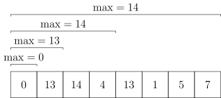
A sparse table (Sparse Table, ST table) is a data structure for solving idempotent range-query problems.

Introduction

Consider the brute-force approach: scan the interval $[l,r]$ once for every query and find its maximum.

Clearly, this algorithm will time out.

Sparse table

Based on the idea of binary lifting, a sparse table can preprocess in $\Theta(n\log n)$ time and answer each query in $\Theta(1)$ time. However, it does not support updates.

Based on binary lifting, consider how to find an interval maximum. If we follow the usual binary-lifting procedure and jump $2^i$ steps at a time, the query complexity is still $\Theta(\log n)$, which is no better than a segment tree, while one preprocessing step is even slower than for a segment tree.

Observe that $\max(x,x)=x$; in other words, interval maximum is an idempotent contribution problem. Even if the preprocessed intervals used to answer a query overlap, as long as their union is the queried interval, the final answer is correct.

A manual simulation shows that at most two preprocessed intervals can cover a query interval. Thus, the query complexity can be reduced to $\Theta(1)$, which is very effective for problems with many queries.

The implementation is as follows.

Let $f(i,j)$ denote the maximum on interval $[i,i+2^j-1]$.

Clearly, $f(i,0)=a_i$.

By the definition, the second dimension is equivalent to "jumping $2^j-1$ steps" during binary lifting. Following the binary-lifting idea, we obtain the transition: $f(i,j)=\max(f(i,j-1),f(i+2^{j-1},j-1))$.

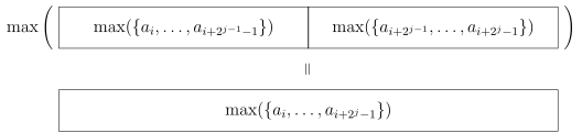
That is the preprocessing part. A query can be implemented simply as follows.

For each query $[l,r]$, split it into $[l,l+2^s-1]$ and $[r-2^s+1,r]$, where $s=\left\lfloor\log_2(r-l+1)\right\rfloor$. The maximum of the two results is the answer.

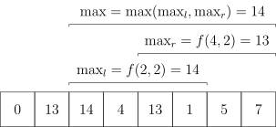
By the argument above for idempotent contribution problems, because maximum is idempotent, the overlap does not affect the interval maximum. Since these two intervals completely cover $[l,r]$, the answer is correct.

#include <algorithm>
#include <iostream>
using namespace std;
constexpr int N = 100000 + 5;
constexpr int logN = 16;  // ⌊ log_2 N ⌋
int f[logN + 1][N], Logn[N];

// initialize logarithm values
void pre() {
  Logn[2] = 1;
  for (int i = 3; i < N; i++) {
    Logn[i] = Logn[i / 2] + 1;
  }
}

int main() {
  cin.tie(nullptr)->sync_with_stdio(false);
  pre();
  int n, m;
  cin >> n >> m;
  for (int i = 1; i <= n; i++) cin >> f[0][i];
  for (int j = 1; j <= logN; j++)
    for (int i = 1; i + (1 << j) - 1 <= n; i++)
      f[j][i] = max(f[j - 1][i], f[j - 1][i + (1 << (j - 1))]);  // specific ST table implementation
  for (int i = 1; i <= m; i++) {
    int x, y;
    cin >> x >> y;
    int s = Logn[y - x + 1];
    cout << max(f[s][x], f[s][y - (1 << s) + 1]) << '\n';
  }
  return 0;
}

#include <algorithm>
#include <functional>
#include <iostream>
#include <vector>
#if defined(_MSC_VER) && !defined(__clang__)
#include <immintrin.h>
#define __builtin_clz _lzcnt_u32
#endif
using namespace std;

// use a built-in function to compute ⌊ log_2 x ⌋
int lg2(int x) { return 31 - __builtin_clz(x); }

template <typename T>
class SparseTable {
  using VT = vector<T>;
  using VVT = vector<VT>;
  using func_type = function<T(const T &, const T &)>;

  VVT ST;

  static T default_func(const T &t1, const T &t2) { return max(t1, t2); }

  func_type op;

 public:
  SparseTable(const vector<T> &v, func_type _func = default_func) {
    op = _func;
    int n = v.size(), l = lg2(n);
    ST.assign(l + 1, VT(n, 0));
    for (int i = 0; i < n; ++i) {
      ST[0][i] = v[i];
    }
    for (int j = 1; j <= l; ++j) {
      for (int i = 0; i + (1 << j) <= n; ++i) {
        ST[j][i] = op(ST[j - 1][i], ST[j - 1][i + (1 << (j - 1))]);
      }
    }
  }

  T query(int l, int r) {
    int q = lg2(r - l + 1);
    return op(ST[q][l], ST[q][r - (1 << q) + 1]);
  }
};

int main() {
  cin.tie(nullptr)->sync_with_stdio(false);
  int n, m;
  cin >> n >> m;
  vector<int> a(n);
  for (int &i : a) cin >> i;
  SparseTable<int> st(a);
  for (int i = 1; i <= m; ++i) {
    int x, y;
    cin >> x >> y;
    cout << st.query(x - 1, y - 1) << '\n';
  }
  return 0;
}

import sys

input = sys.stdin.readline


class SparseTable:
    def __init__(self, arr: list, func=min):
        self.func = func
        self.n = len(arr)
        self.log = [0] * (self.n + 1)

        for i in range(2, self.n + 1):
            self.log[i] = self.log[i // 2] + 1

        self.k = self.log[self.n]
        self.st = [[0] * (self.n) for _ in range(self.k + 1)]
        self.st[0] = arr

        for j in range(1, self.k + 1):
            i = 0
            while i + (1 << j) <= self.n:
                self.st[j][i] = self.func(
                    self.st[j - 1][i], self.st[j - 1][i + (1 << (j - 1))]
                )
                i += 1

    def query(self, left: int, right: int):
        j = self.log[right - left + 1]
        return self.func(self.st[j][left], self.st[j][right - (1 << j) + 1])


n, m = map(int, input().split())
a = list(map(int, input().split()))
st = SparseTable(a, max)
for _ in range(m):
    left, right = map(int, input().split())
    print(st.query(left - 1, right - 1))

Points to note

1. Input and output data are usually large, so enabling I/O optimizations is recommended.

2. When preprocessing a sparse table, an array usually has one dimension of size $\log n$ and another of size $n$. The dimension of size $\log n$ should preferably be the first dimension to improve cache locality.

3. Recomputing logarithms with std::log for every query is not worthwhile. Use built-ins such as __builtin_clz or __lg instead. If these built-ins cannot be used, precompute the logarithms as follows:

Maintaining other information with a sparse table

Besides RMQ, there are other idempotent contribution problems. For example, sparse tables can efficiently solve interval bitwise AND, interval bitwise OR, and interval GCD.

Note that for interval GCD, the sparse-table query complexity is not better than that of a segment tree. Let the value range be $w$: the sparse-table query complexity is $\Theta(\log w)$, while the segment-tree complexity is $\Theta(\log n+\log w)$ (and the value range is generally larger than $n$). However, the sparse-table preprocessing complexity is no worse than the segment tree's, and a sparse table is much simpler to implement.

If we analyze them, idempotent contribution problems generally contain some component analogous to RMQ. For example, interval bitwise AND takes the minimum independently at each bit, while interval GCD takes the minimum exponent for each prime factor.

Summary

A sparse table maintains interval information for idempotent operations (which must also be associative) with low time complexity and relatively little code compared with other algorithms. However, the information a sparse table can maintain is very limited, it is not easy to extend, and it does not support updates.

Exercises

• SCOI2007 Rainfall

• [USACO07JAN] Balanced Lineup

Appendix: time-complexity analysis of interval GCD with a sparse table

During the algorithm, there may be $\Theta(\log n)$ iterations. Each iteration may recursively call the GCD function. Let the value range be $w$; the GCD function has worst-case time complexity $\Omega(\log w)$, so the apparent total complexity is $O(n\log n\log w)$.

However, during the GCD process, every recursive call except the last reduces some number in the sequence by at least half. The numbers in the sequence can be halved at most $\log_2 (w^n)=\Theta(n\log w)$ times in total, so the recursive part of GCD runs at most $O(n\log w)$ times. Adding the $\Theta(n\log n)$ loop portion (and the final recursion level), the total complexity is $O(n(\log w+\log n))$. Since data can be constructed to achieve $\Omega(n(\log w+\log n))$, the final complexity is $\Theta(n(\log w+\log n))$.

The query complexity is easy to analyze. In the worst case, every query asks for the worst pair of numbers, giving complexity $\Theta(\log w)$. Therefore, maintaining interval GCD with a sparse table has preprocessing complexity $\Theta(n(\log n+\log w))$ and single-query complexity $\Theta(\log w)$.

The corresponding segment-tree operations have preprocessing complexity $\Theta(n\log w)$ and single-query complexity $\Theta(\log n+\log w)$.

This is not a rigorous mathematical proof. A more rigorous proof is given below: