AIOJ

The time required by the same algorithm varies somewhat on different computers, and its actual running time is difficult to calculate theoretically; measuring it directly is also troublesome. Therefore, we usually consider not the actual time required by the algorithm, but the number of basic operations it needs to perform.

Time complexity and space complexity are important criteria for measuring the efficiency of an algorithm.

Number of basic operations

On an ordinary computer, addition, subtraction, multiplication, division, accessing variables (variables of basic data types, the same below), assigning values to variables, and so on can all be regarded as basic operations.

Counting or estimating the number of basic operations can serve as an indicator for evaluating an algorithm's running time.

Time complexity

Definition

When measuring how fast an algorithm is, the size of the data must be considered. Data size generally refers to the number of input numbers, the number of vertices and edges in a graph given in the input, and so on. In general, the larger the data size, the longer the algorithm takes. In algorithm competitions, when measuring an algorithm's efficiency, the most important thing is not its running time at a particular data size, but the trend in which its running time grows with the data size, namely time complexity.

Introduction

There are several main reasons for considering the trend of running time as the data size changes:

Modern computers can perform hundreds of millions or more basic operations per second, so the data sizes we process are usually very large. If algorithm A takes $n$ time on data of size $100n$ , while algorithm B takes $n$ time on data of size $n^2$ , then when the data size is less than $100$ , algorithm B takes less time; however, within one second algorithm A can process data of size millions, whereas algorithm B can process only data of size tens of thousands. When algorithms are allowed to run for longer, the impact of time complexity on the processable data size becomes more apparent, far exceeding the impact of running time at the same data size.
We use the number of basic operations to represent an algorithm's running time, but different basic operations take different amounts of actual time; for example, addition and subtraction take far less time than division. Ignoring the differences between different basic operations and between one basic operation and ten basic operations when calculating time complexity eliminates the effect of differing operation times.

Of course, an algorithm's running time is not determined entirely by the input size; it is also related to the input's contents. Therefore, time complexity is further divided into several kinds, for example:

Worst-case time complexity, namely the time complexity corresponding to the input that takes the longest time for each input size. In algorithm competitions, since the input can be chosen arbitrarily within the given data range, we generally consider worst-case time complexity to ensure that an algorithm can pass any data within a given range.
Average (expected) time complexity, namely the complexity of the average running time over all possible inputs for each input size (the complexity of the expected running time under random input).

The so-called "trend of running time as the data size grows" is a vague concept. We need to use the asymptotic notation introduced below to express time complexity formally.

Definition of asymptotic notation

Asymptotic notation is a standard description of the order of a function. Simply put, asymptotic notation ignores the slower-growing parts of a function and the coefficients of its terms (in time-complexity analysis, coefficients are generally called "constants"), while retaining the important parts that can indicate the function's growth trend.

A simple way to remember this is that notation containing equality (non-strict) uses uppercase letters, while notation without equality (strict) uses lowercase letters: equality is $\Theta$ , less than is $O$ , and greater than is $\Omega$ . Big $O$ and little $o$ were originally the Greek letter Omicron; because their shapes are the same, they can also be understood as uppercase $O$ and lowercase $o$ in the Latin alphabet.

In English, the roots "-micro-" and "-mega-" are commonly used to denote the negative sixth power of 10 (one millionth) and the sixth power (one million), and also "small" and "large". Small and large are also meanings commonly represented by the Greek letters Omicron and Omega.

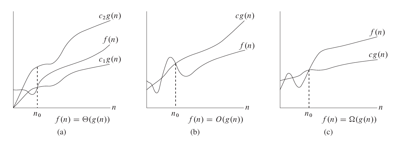
Big Theta notation

For functions $f(n)$ and $g(n)$ , $f(n)=\Theta(g(n))$ if and only if $\exists c_1,c_2,n_0>0$ , such that $\forall n \ge n_0, 0\le c_1\cdot g(n)\le f(n) \le c_2\cdot g(n)$ .

That is, if $f(n)=\Theta(g(n))$ , then we can find two positive numbers $c_1, c_2$ such that $f(n)$ is bounded between $c_1\cdot g(n)$ and $c_2\cdot g(n)$ .

For example, $3n^2+5n-3=\Theta(n^2)$ ; here, $c_1, c_2, n_0$ can be $2, 4, 100$ , respectively. $n\sqrt {n} + n{\log^5 n} + m{\log m} +nm=\Theta(n\sqrt {n} + m{\log m} + nm)$ ; here, $c_1, c_2, n_0$ can be $1, 2, 100$ , respectively.

Big O notation

The $\Theta$ notation gives both an upper and a lower asymptotic bound for a function. If we know only an asymptotic upper bound and not an asymptotic lower bound, we can use $O$ notation. $f(n)=O(g(n))$ if and only if $\exists c,n_0$ , such that $\forall n \ge n_0,0\le f(n)\le c\cdot g(n)$ .

When studying time complexity, $O$ notation is usually used because we are generally concerned with the upper bound on a program's running time, not its lower bound.

It should be noted that the "upper bound" and "lower bound" here refer to the function's growth trend, not to the algorithm. The upper bound on an algorithm's running time corresponds to its "worst-case time complexity", rather than Big $O$ notation. Therefore, it is entirely valid to use $\Theta$ notation to express worst-case time complexity; one could even say that $\Theta$ is more precise than $O$ . The main reasons for using $O$ notation are, first, that sometimes we can prove only an upper bound on the time complexity and not its lower bound (which generally occurs for more complicated algorithms and complexity analyses), and second, that $O$ is more convenient to type on a computer.

Big Omega notation

Similarly, we use $\Omega$ notation to describe a function's asymptotic lower bound. $f(n)=\Omega(g(n))$ if and only if $\exists c,n_0$ , such that $\forall n \ge n_0,0\le c\cdot g(n)\le f(n)$ .

Little o notation

If $O$ notation is equivalent to the less-than-or-equal-to sign, then $o$ notation is equivalent to the less-than sign.

Little $o$ notation is widely used in mathematical analysis. The Taylor expansion of a function at a point has a Peano remainder, and little $o$ notation expresses strict less-than, thereby enabling asymptotic analysis of equivalent infinitesimals.

$f(n)=o(g(n))$ if and only if, for any given positive number $c$ , $\exists n_0$ , such that $\forall n \ge n_0,0\le f(n)< c\cdot g(n)$ .

Little omega notation

If $\Omega$ notation is equivalent to the greater-than-or-equal-to sign, then $\omega$ notation is equivalent to the greater-than sign.

$f(n)=\omega(g(n))$ if and only if, for any given positive number $c$ , $\exists n_0$ , such that $\forall n \ge n_0,0\le c\cdot g(n)< f(n)$ .

Common properties

$f(n) = \Theta(g(n))\iff f(n)=O(g(n))\land f(n)=\Omega(g(n))$
$f_1(n) + f_2(n) = O(\max(f_1(n), f_2(n)))$
$f_1(n) \times f_2(n) = O(f_1(n) \times f_2(n))$
$\forall a \neq 1, \log_a{n} = O(\log_2 n)$ . The change-of-base formula shows that any logarithmic function has the same growth rate regardless of its base, so the base of a logarithm is generally omitted in asymptotic time complexity.

Examples of simple time-complexity calculations

`for` loop

C++

int n, m;
std::cin >> n >> m;
for (int i = 0; i < n; ++i) {
  for (int j = 0; j < n; ++j) {
    for (int k = 0; k < m; ++k) {
      std::cout << "hello world\n";
    }
  }
}

Python

n = int(input())
m = int(input())
for i in range(0, n):
    for j in range(0, n):
        for k in range(0, m):
            print("hello world")

Java

int n, m;
n = input.nextInt();
m = input.nextInt();
for (int i = 0; i < n; ++i) {
    for (int j = 0; j < n; ++j) {
        for (int k = 0; k < m; ++k) {
            System.out.println("hello world");
        }
    }
}

If the sizes of input values $n$ and $m$ are used as the data size, the time complexity of the code above is $\Theta(n^2m)$ .

DFS

When performing DFS on a graph with $n$ vertices and $m$ edges, because each vertex and each edge is visited only a constant number of times, the complexity is $\Theta(n+m)$ .

Which quantities are constants?

When we need to perform several operations, how do we determine whether these operations affect the time complexity? For example:

C++

constexpr int N = 100000;
for (int i = 0; i < N; ++i) {
  std::cout << "hello world\n";
}

Python

N = 100000
for i in range(0, N):
    print("hello world")

Java

final int N = 100000;
for (int i = 0; i < N; ++i) {
    System.out.println("hello world");
}

If the size of $N$ is not regarded as the input size, the time complexity of this code is $O(1)$ .

When calculating time complexity, it is important which variables are regarded as the input size. All quantities unrelated to the input size are regarded as constants and can be treated as $1$ when calculating complexity.

It should be noted that in theoretical discussions related to time complexity, "an algorithm can solve problems of any size" is a basic assumption (of course, in practice, problems that are too large cannot be solved because time and storage space are limited). Therefore, solving problems with a limited data size in constant time (for example, precomputing the answer for every possible input in the data range) cannot make an algorithm's time complexity become $O(1)$ .

Master Theorem

We can use the Master Theorem to quickly find the complexity of recursive algorithms. The recurrence relation of the Master Theorem is as follows:

T(n) = a T\left(\frac{n}{b}\right)+f(n)\qquad \forall n > b

Then

T(n) = \begin{cases}\Theta(n^{\log_b a}) & f(n) = O(n^{\log_b (a)-\epsilon}),\epsilon > 0 \\ \Theta(f(n)) & f(n) = \Omega(n^{\log_b (a)+\epsilon}),\epsilon\ge 0\\ \Theta(n^{\log_b a}\log^{k+1} n) & f(n)=\Theta(n^{\log_b a}\log^k n),k\ge 0 \end{cases}

It should be noted that the second case here also needs to satisfy the regularity condition, that is, $a f(n/b) \leq c f(n)$ , for some constant $c < 1$ and sufficiently large $n$ .

The proof idea is to decompose a problem of size $n$ into $a$ problems of size $(\frac{n}{b})$ , and then merge them successively until reaching the top level. Each time subproblems are merged, $f(n)$ time is required.

Proof

Based on the proof idea mentioned above, the detailed proof is as follows.

At level $0$ (the top level), merging the subproblems takes $f(n)$ time.

At level $1$ (the subproblems produced by the first division), there are $a$ subproblems, and merging each subproblem takes $f\left(\frac{n}{b}\right)$ time, so merging all of them takes $a f\left(\frac{n}{b}\right)$ time.

Recursing level by level, we can write the recursion tree as follows:

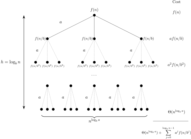
This tree has height ${\log_b n}$ and $n^{\log_b a}$ leaves, so $T(n) = \Theta(n^{\log_b a}) + g(n)$ , where $g(n) = \sum_{j = 0}^{\log_{b}{n - 1}} a^{j} f(n / b^{j})$ .

For the first case: $f(n) = O(n^{\log_b a-\epsilon})$ , so $g(n) = O(n^{\log_b a})$ .

For the second case: first, $g(n) = \Omega(f(n))$ . Also, because $a f(\dfrac{n}{b}) \leq c f(n)$ , as long as $c$ is a sufficiently small positive number and $n$ is sufficiently large, we can deduce that $g(n) = O(f(n)$ . By squeezing between the two sides, we obtain $g(n) = \Theta(f(n))$ .

For the third case: $f(n) = \Theta(n^{\log_b a})$ , so $g(n) = O(n^{\log_b a} {\log n})$ . The result for $T(n)$ follows immediately once $g(n)$ is obtained.

The following examples illustrate how to use the Master Theorem.

$T(n) = 2T\left(\frac{n}{2}\right) + 1$ , so $a=2, b=2, {\log_2 2} = 1$ . Then $\epsilon$ can take a value in $(0, 1]$ , satisfying the first case, so $T(n) = \Theta(n)$ .
$T(n) = T\left(\frac{n}{2}\right) + n$ , so $a=1, b=2, {\log_2 1} = 0$ . Then $\epsilon$ can take a value in $(0, 1]$ , satisfying the second case, so $T(n) = \Theta(n)$ .
$T(n) = T\left(\frac{n}{2}\right) + {\log n}$ , so $a=1, b=2, {\log_2 1}=0$ . Then $k$ can take the value $1$ , satisfying the third case, so $T(n) = \Theta(\log^2 n)$ .
$T(n) = T\left(\frac{n}{2}\right) + 1$ , so $a=1, b=2, {\log_2 1} = 0$ . Then $k$ can take the value $0$ , satisfying the third case, so $T(n) = \Theta(\log n)$ .

Amortized complexity

See Amortized complexity for details.

Space complexity

Similarly, the trend in which the space used by an algorithm changes with the input size can be measured by space complexity.

Computational complexity

This article has introduced complexity mainly from the perspective of algorithm analysis. If you are interested, you can learn more at Computational complexity.

Introduction to Complexity