Prefix Sums & Difference Arrays

Introduction

Prefix sums and difference arrays are commonly used techniques in algorithm competitions: the former is used to quickly compute interval sums, while the latter is used to perform interval updates efficiently.

Prefix Sums

A prefix sum can be understood simply as "the sum of the first $n$ terms of a sequence". It is an important preprocessing technique.

One-dimensional Prefix Sums

For a sequence of length $n$, $\{a_i\}$, if we need to query the sum of the sequence values in an interval $[l,r]$ repeatedly, we can consider using prefix sums. The prefix sums of the sequence are

They can be computed term by term using the recurrence

To query the sum of the sequence in the interval $[l,r]$, we only need to compute the difference

Thus, after $O(n)$-time preprocessing, the complexity of a single interval-sum query is reduced to $O(1)$.

int n;                // Array size.
std::vector<int> a;   // Array. (indexed from 1)
std::vector<int> ps;  // Prefix sum array.

// Calculate prefix sum.
void prefix_sum() {
  ps = a;
  // Or simply:
  // std::partial_sum(a.begin(), a.end(), ps.begin());
  for (int i = 1; i <= n; ++i) {
    ps[i] += ps[i - 1];
  }
}

// Query sum of elements in [l, r].
int query(int l, int r) { return ps[r] - ps[l - 1]; }

n = 0  # Array size
a = []  # Array (indexed from 1)
ps = []  # Prefix sum array


# Calculate prefix sum
def prefix_sum():
    global ps
    ps = a[:]
    # Or simply:
    # ps = list(itertools.accumulate(a))
    for i in range(1, n + 1):
        ps[i] += ps[i - 1]


# Query sum of elements in [l, r]
def query(l, r):
    return ps[r] - ps[l - 1]

The C++ standard library implements the prefix-sum function std::partial_sum, which is defined in the <numeric> header. Starting from C++17, the standard library also provides std::inclusive_scan, a prefix-sum function with the same functionality, also defined in <numeric>.

Two-dimensional/Multidimensional Prefix Sums

Extending one-dimensional prefix sums to multiple dimensions gives multidimensional prefix sums. There are two common methods for computing multidimensional prefix sums.

Based on the Inclusion-Exclusion Principle

This method is mostly used for two-dimensional prefix sums. Given a two-dimensional array of size $m\times n$, denoted by $A$, we want to compute its prefix sums $S$. Then $S$ is also a two-dimensional array of size $m\times n$, and

By analogy with the one-dimensional case, $S_{i,j}$ should be computable from $S_{i-1,j}$ or $S_{i,j-1}$, avoiding repeated computation of the sums of earlier terms. However, if we directly add $S_{i-1,j}$ and $S_{i,j-1}$ and then add $A_{i,j}$, the prefix sum of the overlapping part $S_{i-1,j-1}$ is counted twice, so this part must also be subtracted. This is the inclusion-exclusion principle. Thus, we obtain the recurrence

In the implementation, simply iterate over $(i,j)$ and compute the sums.

Example

Consider a concrete example.

Here, $S$ is the prefix sum of matrix $A$. By definition, $S_{3,3}$ is the sum of the submatrix inside the dashed box in the left image. Also, $S_{3,2}$ is the sum of the blue submatrix, $S_{2,3}$ is the sum of the red submatrix, and the sum of their overlapping part is $S_{2,2}$. It is clear that directly adding $S_{3,2}$ and $S_{2,3}$ counts $S_{2,2}$ twice, so we have

$$S_{3,3} = A_{3,3} + S_{2,3} + S_{3,2} - S_{2,2} = 5 + 18 + 15 - 9 = 29.$$

Similarly, after preprocessing the two-dimensional prefix sums, to query the sum of a submatrix whose upper-left corner is $(i_1,j_1)$ and lower-right corner is $(i_2,j_2)$, compute

This can be done in $O(1)$ time.

In two dimensions, the time complexity of the above algorithm can simply be considered $O(mn)$, which is linear in the size of the given array. However, when the dimension $k$ increases, the number of terms involved in the inclusion-exclusion principle grows exponentially, and the time complexity becomes $O(2^kN)$, where $k$ is the array dimension and $N$ is the size of the given array. Therefore, this algorithm is no longer applicable.

#include <algorithm>
#include <iostream>
#include <vector>

// --8<-- [start:core]
int n, m;
std::vector<std::vector<int>> a, ps;  // (n + 1) x (m + 1).

// Calculate the prefix sum of 2-d array.
void prefix_sum() {
  ps = a;
  for (int i = 1; i <= n; ++i)
    for (int j = 1; j <= m; ++j)
      ps[i][j] += ps[i - 1][j] + ps[i][j - 1] - ps[i - 1][j - 1];
}

// Find the sum of elements in submatrix [x1, y1] to [x2, y2].
int query(int x1, int y1, int x2, int y2) {
  return ps[x2][y2] - ps[x1 - 1][y2] - ps[x2][y1 - 1] + ps[x1 - 1][y1 - 1];
}

// --8<-- [end:core]
int main() {
  std::cin >> n >> m;
  a.assign(n + 1, std::vector<int>(m + 1));

  for (int i = 1; i <= n; i++)
    for (int j = 1; j <= m; j++) std::cin >> a[i][j];

  prefix_sum();

  int ans = 0;
  for (int l = 1; l <= std::min(n, m); ++l)
    for (int i = l; i <= n; i++)
      for (int j = l; j <= m; j++)
        if (query(i - l + 1, j - l + 1, i, j) == l * l) ans = std::max(ans, l);

  std::cout << ans << std::endl;
  return 0;
}

# --8<-- [start:core]
n, m = 0, 0
a = []  # (n+1) x (m+1)
ps = []  # prefix sum array


# Calculate the prefix sum of 2D array.
def prefix_sum():
    global ps
    ps = [row[:] for row in a]  # Deep copy of a
    for i in range(1, n + 1):
        for j in range(1, m + 1):
            ps[i][j] += ps[i - 1][j] + ps[i][j - 1] - ps[i - 1][j - 1]


# Find the sum of elements in submatrix [x1, y1] to [x2, y2].
def query(x1, y1, x2, y2):
    return ps[x2][y2] - ps[x1 - 1][y2] - ps[x2][y1 - 1] + ps[x1 - 1][y1 - 1]


# --8<-- [end:core]
if __name__ == "__main__":
    n, m = map(int, input().split())

    # Initialize with zero padding for 1-based indexing
    a = [[0] * (m + 1)]
    for _ in range(n):
        row = list(map(int, input().split()))
        a.append([0] + row)

    prefix_sum()
    ans = 0

    for l in range(1, min(n, m) + 1):
        for i in range(l, n + 1):
            for j in range(l, m + 1):
                if query(i - l + 1, j - l + 1, i, j) == l * l:
                    ans = max(ans, l)

    print(ans)

Dimension-by-dimension Prefix Sums

In the general case, given a $k$-dimensional array $A$ of size $N$, we likewise want to compute its prefix sums $S$. Here,

The formula above shows that a $k$-dimensional prefix sum is equal to performing $k$ summations. Therefore, a straightforward algorithm is to consider one dimension at a time, fix all other dimensions, and compute several one-dimensional prefix sums. After summing along all $k$ dimensions, we obtain the $k$-dimensional prefix sums.

int N1, N2, N3;
std::vector<std::vector<std::vector<int>>> a,
    ps;  // (N1 + 1) x (N2 + 1) x (N3 + 1).

// Calculate prefix sum of 3d array.
void prefix_sum() {
  ps = a;

  // Prefix-sum for 3rd dimension.
  for (int i = 1; i <= N1; ++i)
    for (int j = 1; j <= N2; ++j)
      for (int k = 1; k <= N3; ++k) ps[i][j][k] += ps[i][j][k - 1];

  // Prefix-sum for 2nd dimension.
  for (int i = 1; i <= N1; ++i)
    for (int j = 1; j <= N2; ++j)
      for (int k = 1; k <= N3; ++k) ps[i][j][k] += ps[i][j - 1][k];

  // Prefix-sum for 1st dimension.
  for (int i = 1; i <= N1; ++i)
    for (int j = 1; j <= N2; ++j)
      for (int k = 1; k <= N3; ++k) ps[i][j][k] += ps[i - 1][j][k];
}

Because each dimension is considered by traversing the entire array only once, the complexity of this algorithm is $O(kN)$, which is usually acceptable.

Special Case: Sum over Subsets DP

A relatively large dimension often occurs in a class of problems called sum over subsets (SOS) problems. This is a special case of high-dimensional prefix sums.

The problem is described as follows. Consider a set of size $n$ and a function $f$ defined on all of its subsets. We want to compute its sum-over-subsets function $g$, which satisfies

That is, $g(S)$ equals the sum, over all subsets $T\subseteq S$, of the corresponding function values $f(T)$.

First, the sum-over-subsets problem can be written in the form of high-dimensional prefix sums. Notice that the subsets of $S$ can be represented as a length-$n$ binary string $s$ using the idea of state compression. Regard each bit of the string as one dimension of an array. Then $f$ is actually an $n$-dimensional array, and the index in each dimension must be in $\{0,1\}$. At the same time, the subset relation is equivalent to the index-order relation:

Therefore, summing over subsets is exactly computing the prefix sums of this $n$-dimensional array.

Now, we can directly use the dimension-by-dimension prefix-sum method described above to compute the sum over subsets. The time complexity is $O(n2^n)$.

int n;
std::vector<int> a, ps;  // length = 1 << n.

void sum_of_subsets() {
  ps = a;
  // Loop over dimensions.
  for (int i = 0; i < n; ++i) {
    // Loop over i-th dimension.
    for (int st = 0; st < (1 << n); ++st) {
      // This condition implies that i-th dimension is 1.
      if ((st >> i) & 1) {
        // ps[... 1 ...] += ps[... 0 ...]. (i-th dimension)
        ps[st] += ps[st ^ (1 << i)];
      }
    }
  }
}

The inverse operation of sum over subsets requires the inclusion-exclusion principle. The sum-over-subsets problem is also one of the necessary steps of the fast Möbius transform.

Prefix Sums on Trees

One-dimensional prefix sums can also be generalized to the case of a rooted tree (with root $1$). After preprocessing the prefix sums, we can quickly compute the sum of the weights along a path in the tree.

Vertex Weights

First consider the case where weights are stored at vertices. Suppose vertex $x$ has weight $a_x$. Using the recurrence

we can compute the sum of the weights of the vertices on the path from the root to vertex $x$, where $\operatorname{fa}(x)$ denotes the parent of $x$. After preprocessing the prefix sums, the desired path sum can be computed using

This gives the vertex-weight sum along the path connecting vertices $x$ and $y$. Here, $\operatorname{lca}(x, y)$ denotes the lowest common ancestor of vertices $x$ and $y$.

Edge Weights

The case where weights are stored on edges can almost be transformed into the vertex-weight case. For every non-root vertex $x\neq 1$, let $\operatorname{edge}(x)$ denote the edge connecting vertex $x$ and its parent $\operatorname{fa}(x)$. We can assume that the edge weight is stored at the vertex farther from the root. In other words, vertex $x$ stores the weight of edge $\operatorname{edge}(x)$. The root stores weight $0$. Then, using the recurrence discussed in the previous subsection, we can likewise preprocess the path from the root to vertex $x$, whose total edge weight is $S_x$.

In this case, the sum of the vertex weights on the path connecting vertices $x$ and $y$ can be queried by

Unlike the vertex-weight case, the queried sum does not include the weight at $\operatorname{lca}(x, y)$, because the edge weight stored there is not on the path in question.

Subtree Sums

Unlike arrays, a tree is not symmetric from head to tail, so computing "prefix sums" bottom-up (from leaves to the root) and top-down (from the root to the leaves) produces different results. In general, "prefix sums on trees" refers to prefix sums computed top-down. For convenience, this article calls the "prefix sums" computed bottom-up subtree sums.

The sum of vertex weights in the subtree rooted at vertex $x$, namely the corresponding subtree sum, is

Here, $\operatorname{desc}(x)$ denotes the set of all descendants of $x$, including itself.

Unlike prefix sums on trees, subtree sums cannot be used to compute path sums in $O(1)$, but they are useful for understanding tree difference arrays below.

Difference Arrays

Difference arrays are a strategy complementary to prefix sums and are the inverse operation of prefix sums. In competitions, it is more common to maintain information about a difference sequence to perform multiple interval updates than to compute the difference array of a given sequence. After all interval updates are complete, the original sequence can be recovered using prefix sums, allowing queries on the original sequence. Note that update operations must be performed before query operations.

If mixed updates and queries must be supported, use a Fenwick tree, but the underlying ideas are shared.

One-dimensional Difference Arrays

For a sequence $\{a_i\}$, its difference sequence $\{D_i\}$ is defined by

The C++ standard library implements the difference function std::adjacent_difference, which is defined in the <numeric> header.

The relationship between prefix sums and difference arrays is as follows:

Difference information is often used to maintain multiple operations that add a number to an interval of a sequence, followed by one or more queries for the value at a position in the sequence.

Suppose we want to add a number to every element of sequence $\{a_i\}$ in the interval $[l,r]$; let that number be $v$. We can perform the following operations on its difference sequence $\{D_i\}$:

After all update operations are complete, the values of the updated sequence $\{a_i\}$ can be recovered using a prefix-sum operation. A single update takes $O(1)$ time. When querying, perform one $O(n)$ prefix-sum operation, after which each query takes $O(1)$ time.

int n;
std::vector<int> diff, a;

// Add v to each element in [l, r].
void add(int l, int r, int v) {
  diff[l] += v;
  if (r < n) diff[r + 1] -= v;
}

// Execute this after all modifications and before all queries.
void prefix_sum() {
  for (int i = 1; i <= n; ++i) a[i] = a[i - 1] + diff[i];
}

Two-dimensional/Multidimensional Difference Arrays

Difference arrays can likewise be generalized to multiple dimensions. Viewing multidimensional differences as the inverse operation of multidimensional prefix sums, computing a multidimensional difference array is equivalent to recovering the original array from its multidimensional prefix sums. As discussed above, the inclusion-exclusion principle can be used. For example, the definition of the two-dimensional difference array is

However, when computing the entire difference array, a simpler and more efficient method is to take differences dimension by dimension: enumerate all dimensions and compute the difference of the array along each dimension once.

Two-dimensional difference information is often used to maintain multiple rectangle-add operations on a two-dimensional array. For example, for the matrix whose upper-left corner is $(x_1,y_1)$ and lower-right corner is $(x_2,y_2)$, to add $v$ to every number, perform the following operations on its difference array $\{D_{i,j}\}$:

After all update operations are complete, a single two-dimensional prefix-sum pass suffices to quickly query values in the updated array.

int n, m;
std::vector<std::vector<int>> diff, a;

// Add v to each element from [x1, y1] to [x2, y2].
void add(int x1, int y1, int x2, int y2, int v) {
  diff[x1][y1] += v;
  if (x2 < n) diff[x2 + 1][y1] -= v;
  if (y2 < m) diff[x1][y2 + 1] -= v;
  if (x2 < n && y2 < m) diff[x2 + 1][y2 + 1] += v;
}

// Execute this after all modifications and before all queries.
void prefix_sum() {
  a = diff;

  for (int i = 1; i <= n; ++i)
    for (int j = 1; j <= m; ++j) a[i][j] += a[i - 1][j];

  for (int i = 1; i <= n; ++i)
    for (int j = 1; j <= m; ++j) a[i][j] += a[i][j - 1];
}

The same idea also works for dimension $k>2$, but a single update takes $O(2^k)$ time, so it becomes impractical as $k$ increases.

Tree Difference Arrays

Difference arrays can be generalized to rooted trees, where they implement interval additions along paths. Depending on whether the maintained information is stored at vertices or edges, tree difference arrays can be divided into vertex differences and edge differences, with slightly different implementations. In contrast to tree prefix-sum operations, it is more common to compute subtree sums after all updates and then query the result. This is the case discussed in this section.

Vertex Differences

To add a value to every vertex weight on the path between vertices $x$ and $y$, let that value be $v$; perform the following operations on its difference sequence $\{D_x\}$:

After all updates are complete, compute the subtree sums once to obtain the updated vertex weights.

Example

When adding a value to the vertex weights on the path between vertices $S$ and $T$, the first two lines of the formula above perform one-dimensional difference operations on the path inside the blue box, and the last two perform one-dimensional difference operations on the path inside the red box:

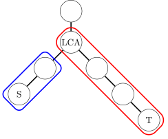
Summing from bottom to top is equivalent to computing prefix sums on these two intervals from bottom to top. Comparing this with the one-dimensional difference operations above makes the correctness of vertex differences clear.

Edge Differences

To add a value to every edge weight on the path between vertices $x$ and $y$, let that value be $v$; perform the following operations on its difference sequence $\{D_x\}$:

After all updates are complete, compute the subtree sums once to obtain the updated vertex weights.

Example

As shown in the figure, edge differences can be used to solve the problem of adding a value to the edge weights along the red path.

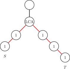
Since performing differences directly on edges is difficult, move the values that should be accumulated on the red edges down to the adjacent vertices; the operation then becomes convenient. Comparing this with the vertex-difference formula makes the edge-difference formula clear.

Example

#include <algorithm>
#include <iostream>
using namespace std;

constexpr int MAXN = 50010;

struct node {
  int to, next;
} edge[MAXN << 1];

int fa[MAXN][30], head[MAXN << 1];
int power[MAXN];
int depth[MAXN], lg[MAXN];
int n, k, ans = 0, tot = 0;

void add(int x, int y) {  // Add an edge
  edge[++tot].to = y;
  edge[tot].next = head[x];
  head[x] = tot;
}

void dfs(int now, int father) {  // DFS to find the maximum pressure
  fa[now][0] = father;
  depth[now] = depth[father] + 1;
  for (int i = 1; i <= lg[depth[now]]; ++i)
    fa[now][i] = fa[fa[now][i - 1]][i - 1];
  for (int i = head[now]; i; i = edge[i].next)
    if (edge[i].to != father) dfs(edge[i].to, now);
}

int lca(int x, int y) {  // Find the LCA, the lowest common ancestor
  if (depth[x] < depth[y]) swap(x, y);
  while (depth[x] > depth[y]) x = fa[x][lg[depth[x] - depth[y]] - 1];
  if (x == y) return x;
  for (int k = lg[depth[x]] - 1; k >= 0; k--) {
    if (fa[x][k] != fa[y][k]) x = fa[x][k], y = fa[y][k];
  }
  return fa[x][0];
}

// Use DFS to find the maximum pressure; add subtree weights during backtracking.
void get_ans(int u, int father) {
  for (int i = head[u]; i; i = edge[i].next) {
    int to = edge[i].to;
    if (to == father) continue;
    get_ans(to, u);
    power[u] += power[to];
  }
  ans = max(ans, power[u]);
}

int main() {
  cin.tie(nullptr)->sync_with_stdio(false);
  cin >> n >> k;
  int x, y;
  for (int i = 1; i <= n; i++) {
    lg[i] = lg[i - 1] + (1 << lg[i - 1] == i);
  }
  for (int i = 1; i <= n - 1; i++) {  // Build the graph
    cin >> x >> y;
    add(x, y);
    add(y, x);
  }
  dfs(1, 0);
  int s, t;
  for (int i = 1; i <= k; i++) {
    cin >> s >> t;
    int ancestor = lca(s, t);
    // Tree difference
    power[s]++;
    power[t]++;
    power[ancestor]--;
    power[fa[ancestor][0]]--;
  }
  get_ans(1, 0);
  cout << ans << '\n';
  return 0;
}

Exercises

Prefix sums:

• Luogu B3612 【Advanced 1, Example 1】 Interval Sum
• Luogu U69096 Inverse of Prefix Sums
• AtCoder joi2007ho_a Maximum Sum
• USACO16JAN Subsequences Summing to Sevens
• USACO05JAN Moo Volume S

Two-dimensional/Multidimensional prefix sums:

• HDU 6514 Monitor
• Luogu P1387 Maximum Square
• HNOI2003 Laser Bomb
• CF 165E Compatible Numbers
• CF 383E Vowels
• ARC 100C Or Plus Max

Prefix sums on trees:

• LOJ 10134.Dis
• LOJ 2491. Sum

Difference arrays:

• Fenwick Tree 3: Range Updates, Range Queries
• Poetize6 IncDec Sequence
• Luogu P4231 Three-step Kill

Two-dimensional/Multidimensional difference arrays:

• Luogu P3397 Carpet
• Luogu P8228 【Wdoi-5】 Modular Nuclear Fusion Furnace

Tree difference arrays:

• Luogu 3128 Maximum Flow
• JLOI2014 Squirrel's New Home
• NOIP2015 Transportation Plan
• NOIP2016 Running Every Day