Fenwick Tree

Introduction

A Fenwick tree is a compact data structure with little code that supports point updates and range queries.

A standard Fenwick tree maintains information and operations that satisfy associativity and support differences, such as addition (sums), multiplication (products), and XOR.

• Associativity: $(x \circ y) \circ z = x \circ (y \circ z)$, where $\circ$ is a binary operator.
• Supporting differences: an operation with an inverse, meaning that given $x \circ y$ and $x$, we can find $y$.

It is important to note:

• For multiplication modulo a modulus to support differences, every number must have an inverse (which is always true when the modulus is prime);
• Information such as $\gcd$ and $\max$ does not support differences, so it cannot be handled by a standard Fenwick tree. However:
  • Two Fenwick trees can be used to handle range minima; see Efficient Range Minimum Queries using Binary Indexed Trees.
  • This page also introduces an extended Fenwick tree that supports queries on non-differentiable information in $\Theta(\log^2n)$ time.

In fact, the problems a Fenwick tree can solve form a subset of those solvable by a segment tree: everything a Fenwick tree can do, a segment tree can certainly do; everything a segment tree can do, a Fenwick tree cannot necessarily do. However, Fenwick-tree code is much shorter than segment-tree code, and its constant factors are smaller, so it is still worth studying.

Sometimes, with the help of a difference array and auxiliary arrays, a Fenwick tree can also solve the stronger problems of range additions with point-value queries and range additions with range-sum queries.

Fenwick tree

First intuition

Let us start with an example: how do we find the prefix sum of $a[1 \ldots 7]$?

One way is to compute $a_1 + a_2 + a_3 + a_4 + a_5 + a_6 + a_7$, which requires summing $7$ numbers.

But what if we know three numbers $A$, $B$, and $C$, where $A = a[1 \ldots 4]$ is a sum, $B = a[5 \ldots 6]$ is a total, and $C = a[7 \ldots 7]$ is a total (which is just $a[7]$ itself)? How would you calculate it? You would certainly answer: $A + B + C$, requiring only the sum of $3$ numbers.

This is why a Fenwick tree can answer queries quickly: we can always split a prefix $[1, n]$ into no more than $\boldsymbol{\log n}$ intervals, so that the information of these $\log n$ intervals is known.

Thus, we only need to combine the information from these $\log n$ intervals to obtain the answer. Compared with directly combining $n$ pieces of information, this is a major improvement in efficiency.

It is easy to see that the information must satisfy associativity; otherwise, it could not be combined as above.

The figure below illustrates how a Fenwick tree works:

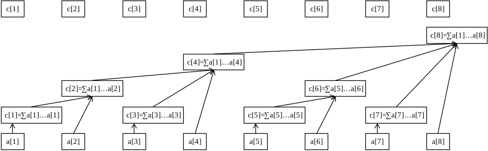
The eight blocks at the bottom represent the original data array $a$. The uneven blocks above (which form the same eight-position array as the top row) represent the parent array of $a$, namely $c$.

The $c$ array stores the sum of a certain interval of the original array $a$; in other words, the information for these intervals is known, and our goal is to decompose a queried prefix into these small intervals.

For example, as the figure shows:

• $c_2$ governs $a[1 \ldots 2]$;
• $c_4$ governs $a[1 \ldots 4]$;
• $c_6$ governs $a[5 \ldots 6]$;
• $c_8$ governs $a[1 \ldots 8]$;
• Every remaining $c[x]$ governs $a[x]$ itself (which can be viewed as the interval $a[x \ldots x]$ of length $1$).

It is easy to see that $c[x]$ always governs an interval whose right endpoint is $x$. We will ignore the left endpoint for now and first build intuition for how a Fenwick tree performs a query.

Example: compute the sum of $a[1 \ldots 7]$.

Process: start at $c_{7}$ and jump backward. We find that $c_{7}$ governs only the element $a_{7}$; then inspect $c_{6}$ and find that $c_{6}$ governs $a[5 \ldots 6]$; then jump to $c_{4}$ and find that $c_{4}$ governs the elements $a[1 \ldots 4]$; finally, we try to jump to $c_0$, but $c_0$ does not actually exist, so we stop.

The $c$ values we found are $c_7, c_6, c_4$. These are exactly the three small intervals into which $a[1 \ldots 7]$ was decomposed, so combining them gives $c_7 + c_6 + c_4$.

Example: compute the sum of $a[4 \ldots 7]$.

Again, we start at $c_7$, jump to $c_6$, and then jump to $c_4$. We now find that it governs the sum of $a[1 \ldots 4]$, but we do not want the $a[1 \ldots 3]$ part. What should we do? Simply subtract the sum of $a[1 \ldots 3]$.

We can instead begin by converting the query for the sum of $a[4 \ldots 7]$ into a query for the sum of $a[1 \ldots 7]$ and a query for the sum of $a[1 \ldots 3]$, then subtract the two results.

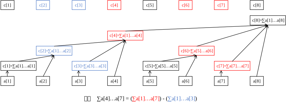
Governed intervals

This raises the question: how far to the left does $c[x](x \ge 1)$ extend? In other words, what is the interval length?

In a Fenwick tree, the interval governed by $c[x]$ is defined to have length $2^{k}$, where:

• If the least significant bit is bit $0$, then $k$ is exactly the bit position in the binary representation of $x$ corresponding to the lowest 1;
• $2^k$ (the length of the interval governed by $c[x]$) is exactly the number formed by the binary representation of $x$'s lowest 1 and all subsequent 0 bits.

For example, which interval does $c_{88}$ govern?

Because $88_{(10)}=01011000_{(2)}$, the lowest 1 and the subsequent 0 bits form the binary number 1000, namely $8$, so $c_{88}$ governs $8$ elements of the $a$ array.

Therefore, $c_{88}$ represents the interval information for $a[81 \ldots 88]$.

Let the number formed by the lowest bits of the binary representation of $x$—the 1 bit and all subsequent 0 bits—be $\operatorname{lowbit}(x)$. Then the interval governed by $c[x]$ is $[x-\operatorname{lowbit}(x)+1, x]$.

How do we compute lowbit? From bitwise operations, we obtain lowbit(x) = x & -x.

int lowbit(int x) {
  // The number formed by the lowest 1 bit of x and all subsequent 0 bits in binary.
  // lowbit(0b01011000) == 0b00001000
  //          ~~~~^~~~
  // lowbit(0b01110010) == 0b00000010
  //          ~~~~~~^~
  return x & -x;
}

def lowbit(x):
    """
    The value formed by the lowest set bit of x and all trailing zeros in its binary representation.
    lowbit(0b01011000) == 0b00001000
            ~~~~~^~~
    lowbit(0b01110010) == 0b00000010
            ~~~~~~~^~
    """
    return x & -x

Range queries

Next, let us examine the concrete operations on a Fenwick tree, starting with range queries.

Recall the process for querying $a[4 \ldots 7]$: we converted it into two subqueries, the sum of $a[1 \ldots 7]$ and the sum of $a[1 \ldots 3]$, and then took their difference.

In fact, every range query can be handled this way: the sum of $a[l \ldots r]$ is the sum of $a[1 \ldots r]$ minus the sum of $a[1 \ldots l - 1]$, converting a range problem into a prefix problem that is easier to handle.

In contests, converting a range query over $l \ldots r$ into two prefix queries over $1 \ldots r$ and $1 \ldots l - 1$, then taking their difference, is a very common technique.

How do we perform a prefix query? Recall the process for querying $a[1 \ldots 7]$:

Jump backward from $c_{7}$: $c_{7}$ governs only the element $a_{7}$; then inspect $c_{6}$ and find that $c_{6}$ governs $a[5 \ldots 6]$; jump to $c_{4}$ and find that $c_{4}$ governs the elements $a[1 \ldots 4]$; then try to jump to $c_0$. But $c_0$ does not actually exist, so we stop.

The $c$ values we found are $c_7, c_6, c_4$. These are exactly the three small intervals into which $a[1 \ldots 7]$ was decomposed; combining them gives $c_7 + c_6 + c_4$.

Observe that at each step we jump to the position immediately to the left of the current interval's left endpoint, making it the right endpoint of the new interval. This is necessary to decompose the prefix without gaps or overlaps. For example, $c_6$ governs $a[5 \ldots 6]$, so the next jump is to $5 - 1 = 4$, accessing $c_4$.

We can write the process for querying $a[1 \ldots x]$ as follows:

• Start from $c[x]$ and jump backward; $c[x]$ governs $a[x-\operatorname{lowbit}(x)+1 \ldots x]$.
• Set $x \gets x - \operatorname{lowbit}(x)$. If $x = 0$, we have reached the end and terminate the loop; otherwise, return to the first step.
• Combine the $c$ values reached.

When implementing this, we do not need to collect all the $c$ values first and combine them afterward; we can combine them while jumping.

For example, if the maintained information is a sum, set the initial $\mathrm{ans} = 0$. Each time we reach a $c[x]$, set $\mathrm{ans} \gets \mathrm{ans} + c[x]$; the final $\mathrm{ans}$ is the result of combining them all.

int getsum(int x) {  // sum of a[1]..a[x]
  int ans = 0;
  while (x > 0) {
    ans = ans + c[x];
    x = x - lowbit(x);
  }
  return ans;
}

def getsum(x):  # sum of a[1]..a[x]
    ans = 0
    while x > 0:
        ans = ans + c[x]
        x = x - lowbit(x)
    return ans

Fenwick-tree properties and its tree structure

Before discussing point updates, let us first explain several basic properties of a Fenwick tree and the origin of its tree structure; this will make point updates easier to understand.

We use the following conventions:

• $l(x) = x - \operatorname{lowbit}(x) + 1$. That is, $l(x)$ is the left endpoint of the range governed by $c[x]$.
• For every positive integer $x$, we can write $x$ in the form $s \times 2^{k + 1} + 2^k$, where $\operatorname{lowbit}(x) = 2^k$.
• The statement “$c[x]$ and $c[y]$ are disjoint” means that the ranges governed by $c[x]$ and $c[y]$ do not intersect, namely that $[l(x), x]$ and $[l(y), y]$ are disjoint. The meaning of statements such as “$c[x]$ is contained in $c[y]$” is analogous.

Property $\boldsymbol{1}$: for $\boldsymbol{x \le y}$, either $\boldsymbol{c[x]}$ and $\boldsymbol{c[y]}$ are disjoint, or $\boldsymbol{c[x]}$ is contained in $\boldsymbol{c[y]}$.

Property $\boldsymbol{2}$: $\boldsymbol{c[x]}$ is strictly contained in $\boldsymbol{c[x + \operatorname{lowbit}(x)]}$.

Property $3$: for any $\boldsymbol{x < y < x + \operatorname{lowbit}(x)}$, $\boldsymbol{c[x]}$ and $\boldsymbol{c[y]}$ are disjoint.

With these three properties in place, we can now examine the tree structure of a Fenwick tree (ignore the edges from $a$ to $c$).

In fact, the tree structure of a Fenwick tree is the graph formed by connecting $x$ to $x + \operatorname{lowbit}(x)$, where $x + \operatorname{lowbit}(x)$ is the parent of $x$.

When considering this tree structure, we ignore the size of the Fenwick tree and regard it as an infinite tree for convenience. In an actual implementation, for $x \le n$ we only use $c[x]$, where $n$ is the length of the original array.

This tree naturally has many useful properties. We list several below (let $fa[u]$ denote the direct parent of $u$):

• $u < fa[u]$．
• $u$ is greater than every descendant of $u$ and less than every ancestor of $u$.
• Node $u$'s $\operatorname{lowbit}$ is strictly less than $fa[u]$'s $\operatorname{lowbit}$.

• The height of node $x$ is $\log_2\operatorname{lowbit}(x)$, namely the bit position in the binary representation of $x$ corresponding to 1.

• $c[u]$ is strictly contained in $c[fa[u]]$ (Property $2$).
• $c[u]$ is strictly contained in $c[v]$, where $v$ is any ancestor of $u$ (by induction on the preceding property).
• $c[u]$ strictly contains $c[v]$, where $v$ is any descendant of $u$ (the preceding property with $u$ and $v$ exchanged).
• For any $v' > u$, if $v'$ is not an ancestor of $u$, then $c[u]$ and $c[v']$ are disjoint.

• For any $v < u$, if $v$ is not in the subtree of $u$, then $c[u]$ and $c[v]$ are disjoint (the preceding property with $u$ and $v'$ exchanged).
• For any $v > u$, the condition that $v$ is an ancestor of $u$ is equivalent to $c[u]$ being strictly contained in $c[v]$ (a summary of the preceding properties). This is the core principle behind Fenwick-tree point updates.
• Let $u = s \times 2^{k + 1} + 2^k$. Then the number of its children is $k = \log_2\operatorname{lowbit}(u)$, and their indices are $u - 2^t(0 \le t < k)$.
  • For example, suppose $k = 3$ and the binary index of $u$ is ...1000. Then $u$ has three children, whose binary indices are ...0111, ...0110, and ...0100.

• The ranges governed by all children of $u$ in $c$ concatenate exactly to $[l(u), u - 1]$.
  • For example, suppose $k = 3$ and the binary index of $u$ is ...1000. Then $u$ has three children, whose binary indices are ...0111, ...0110, and ...0100.
  • c[...0100] represents a[...0001 ~ ...0100].
  • c[...0110] represents a[...0101 ~ ...0110].
  • c[...0111] represents a[...0111 ~ ...0111].
  • It is easy to see that the union of the three ranges above is exactly a[...0001 ~ ...0111], namely $[l(u), u - 1]$.

Point updates

Now let us consider how to perform a point update on $a[x]$.

Our goal is to maintain the $c$ array quickly and correctly. For efficiency, we only need to traverse and update the entries that govern $a[x]$, namely the $c[y]$ values, because the other $c$ values have obviously not changed.

Every entry governing $a[x]$, namely $c[y]$, must contain $c[x]$ (by Property $1$), so $y$ is an ancestor of $x$ in the Fenwick-tree structure. Therefore, we start at $x$ and repeatedly jump to the parent until we pass the length of the original array.

Let $n$ denote the size of $a$. The process for a point update on $a[x]$ is easy to write:

• Initially set $x' = x$.
• Update $c[x']$.
• Set $x' \gets x' + \operatorname{lowbit}(x')$. If $x' > n$, we have reached the end and terminate the loop; otherwise, return to the second step.

The interval information and the type of point update together determine how to update $c[x']$. Here are several examples:

• If $c[x']$ stores a range sum and the update on $a[x]$ adds $p$, then add to every corresponding $c[x']$ the amount $p$.
• If $c[x']$ stores a range product and the update on $a[x]$ multiplies by $p$, then multiply every corresponding $c[x']$ by $p$.

However, the flexibility of point updates means that the update operation and the maintained information need not use the same operation. For example, if $c[x']$ stores a range sum and the update assigns $a[x]$ the value $p$, we can convert it into adding to $a[x]$ the amount $p - a[x]$. If instead it multiplies $a[x]$ by $p$, we can convert it into adding to $a[x]$ the amount $a[x] \times p - a[x]$.

Here is an implementation that maintains range sums with point additions.

void add(int x, int k) {
  while (x <= n) {  // do not go out of bounds
    c[x] = c[x] + k;
    x = x + lowbit(x);
  }
}

def add(x, k):
    while x <= n:  # do not go out of bounds
        c[x] = c[x] + k
        x = x + lowbit(x)

Building the tree

That is, build the Fenwick tree from the original sequence given at the beginning (precomputing all of $c$).

The straightforward method is to convert this into $n$ point updates, with time complexity $\Theta(n \log n)$ (the complexity analysis appears below).

For example, given the sequence $a = (5, 1, 4)$, to build the tree we can treat it as a point addition of $a[1]$ by $5$, a point addition of $a[2]$ by $1$, and a point addition of $a[3]$ by $4$.

There is also an $\Theta(n)$ tree-building method; see Tree building in $\Theta(n)$ on this page.

Complexity analysis

The space complexity is clearly $\Theta(n)$.

Time complexity:

• For a range query: the entire iteration process $x \gets x - \operatorname{lowbit}(x)$ can be viewed as gradually changing, from the lowest bit upward, the binary representation of $x$ so that every $1$ becomes $0$. The number of intervals decomposed equals the number of bit positions at which the binary representation of $x$ has value $1$ (that is, $\operatorname{popcount}(x)$). Therefore, the time complexity of one query is $\Theta(\log n)$.
• For a point update: when jumping to parents, the height of each visited node strictly increases, and $x \le n$ always holds. Since the height of node $x$ is $\log_2\operatorname{lowbit}(x)$, the height reached cannot exceed $\log_2n$, so the number of visited $c$ values is on the order of $\log n$. Therefore, the complexity of one point update is $\Theta(\log n)$.

Range additions with range sums

Prerequisite: prefix sums & differences.

This problem can be solved with two Fenwick trees maintaining a difference array.

Consider sequence $a$'s difference array $d$, where $d[i] = a[i] - a[i - 1]$. Since the prefix sum of the difference array is the original array, $a_i=\sum_{j=1}^i d_j$.

Similarly, we convert a range-sum query into a prefix-sum query using differences. Consider the sum of $a[1 \ldots r]$, namely $\sum_{i=1}^{r} a_i$, and derive it:

Inspecting this expression, it is easy to see that each $d_j$ is added a total of $r - j + 1$ times. Continuing the derivation:

$\sum_{i=1}^r d_i$ does not determine the value of $\sum_{i=1}^r d_i \times i$, so we need two Fenwick trees to maintain the sums of $d_i$ and $d_i \times i$ separately.

How do we perform a range addition? Consider how the original range $a[l \ldots r]$ changes when adding $x$, and how that affects $d$.

Because the difference is $d[i] = a[i] - a[i - 1]$,

• $a[l]$ increases by $v$ while $a[l - 1]$ is unchanged, so $d[l]$ increases by $v$.
• $a[r + 1]$ is unchanged while $a[r]$ increases by $v$, so $d[r + 1]$ decreases by $v$.
• For any positions other than $l$ and $r+1$, namely $i$, either $a[i]$ and $a[i - 1]$ both remain unchanged or both increase by $v$. Thus $a[i] + v - (a[i - 1] + v)$ remains $a[i] - a[i - 1]$, so all other $d[i]$ remain unchanged.

The maintenance method is now clear: in the Fenwick tree maintaining $d_i$, add at $l$ an amount $v$ and at $r + 1$ an amount $-v$; in the Fenwick tree maintaining $d_i \times i$, add at $l$ an amount $v \times l$ and at $r + 1$ an amount $-v \times (r + 1)$.

For the weaker problem of “range addition, point-value query”, it is enough to use a Fenwick tree to maintain one difference array $d_i$. To query the point value at $a[x]$, simply find the sum of $d[1 \ldots x]$.

Here is the code for “range additions with range sums”:

int t1[MAXN], t2[MAXN], n;

int lowbit(int x) { return x & (-x); }

void add(int k, int v) {
  int v1 = k * v;
  while (k <= n) {
    t1[k] += v, t2[k] += v1;
    // Do not write t2[k] += k * v, because k is no longer an index in the original array
    k += lowbit(k);
  }
}

int getsum(int *t, int k) {
  int ret = 0;
  while (k) {
    ret += t[k];
    k -= lowbit(k);
  }
  return ret;
}

void add1(int l, int r, int v) {
  add(l, v), add(r + 1, -v);  // Convert a range addition into two prefix additions
}

long long getsum1(int l, int r) {
  return (r + 1ll) * getsum(t1, r) - 1ll * l * getsum(t1, l - 1) -
         (getsum(t2, r) - getsum(t2, l - 1));
}

t1 = [0] * MAXN
t2 = [0] * MAXN
n = 0


def lowbit(x):
    return x & (-x)


def add(k, v):
    v1 = k * v
    while k <= n:
        t1[k] = t1[k] + v
        t2[k] = t2[k] + v1
        k = k + lowbit(k)


def getsum(t, k):
    ret = 0
    while k:
        ret = ret + t[k]
        k = k - lowbit(k)
    return ret


def add1(l, r, v):
    add(l, v)
    add(r + 1, -v)


def getsum1(l, r):
    return (
        (r) * getsum(t1, r)
        - l * getsum(t1, l - 1)
        - (getsum(t2, r) - getsum(t2, l - 1))
    )

Following this principle, one can implement “range multiplication with range products”, “XOR a number over a range and query the range XOR”, and so on, as long as the maintained information and the range operation use the same operation. Interested readers can try these themselves.

Two-dimensional Fenwick trees

Point updates, submatrix queries

A two-dimensional Fenwick tree, also called a Fenwick tree of Fenwick trees, maintains point updates and prefix information on a two-dimensional array.

As with a one-dimensional Fenwick tree, let $c(x, y)$ denote the total matrix information for $a(x - \operatorname{lowbit}(x) + 1, y - \operatorname{lowbit}(y) + 1) \ldots a(x, y)$; that is, the total information of a matrix with $a(x, y)$ as its lower-right corner, height $\operatorname{lowbit}(x)$, and width $\operatorname{lowbit}(y)$.

For a point update, let:

That is, $f(x, i)$ is the ancestor of $x$ at level $i$ in the Fenwick-tree structure (the level-$0$ ancestor is the node itself).

Then only elements in $c(f(x, i), f(y, j))$ govern $a(x, y)$. When updating $a(x, y)$, we only need to update every $c(f(x, i), f(y, j))$ with $f(x, i) \le n$ and $f(y, j) \le m$.

For a query, let:

Then combine every $c(g(x, i), g(y, j))$ for which $g(x, i), g(y, j) > 0$.

Here is the code for point additions and submatrix-sum queries.

void add(int x, int y, int v) {
  for (int i = x; i <= n; i += lowbit(i)) {
    for (int j = y; j <= m; j += lowbit(j)) {
      // A loop variable must be created here; unlike in a one-dimensional array, we cannot simply write while (x <= n)
      c[i][j] += v;
    }
  }
}

int sum(int x, int y) {
  int res = 0;
  for (int i = x; i > 0; i -= lowbit(i)) {
    for (int j = y; j > 0; j -= lowbit(j)) {
      res += c[i][j];
    }
  }
  return res;
}

int ask(int x1, int y1, int x2, int y2) {
  // Query the submatrix sum
  return sum(x2, y2) - sum(x2, y1 - 1) - sum(x1 - 1, y2) + sum(x1 - 1, y1 - 1);
}

Submatrix additions, submatrix-sum queries

Prerequisites: prefix sums & differences and the range additions with range sums section on this page.

As with the one-dimensional Fenwick-tree problem of range additions with range sums, consider maintaining a difference array.

The difference array of a two-dimensional array is defined as follows:

Thus, for the submatrix whose upper-left corner is $(x_1, y_1)$ and lower-right corner is $(x_2, y_2)$, a submatrix addition of $v$ is equivalent, on the difference array, to adding at $d(x_1, y_1)$ and $d(x_2 + 1, y_2 + 1)$ an amount $v$, and adding at $d(x_2 + 1, y_1)$ and $d(x_1, y_2 + 1)$ an amount $-v$.

As for why this works, write these four $d$ values using their defining formulas and analyze the change in each term.

Consider an example. If the initial difference array is $0$ and the submatrix $a(2, 2) \ldots a(3, 4)$ receives an addition of $v$, the difference array becomes:

(The submatrix $a(2, 2) \ldots a(3, 4)$ is exactly the central matrix of size $2 \times 3$ shown above.)

Therefore, a submatrix addition is implemented as four point additions on the difference array.

Now consider a submatrix-sum query:

For a point $(x, y)$, its two-dimensional prefix sum can be written as:

The reason is that the prefix sum of the prefix sum of the difference array is the original prefix sum.

As with the one-dimensional range-addition/range-sum problem, the number of occurrences of $d(h, k)$ is $(x - h + 1) \times (y - k + 1)$.

Continuing the derivation:

Therefore, we need four Fenwick trees, maintaining the sums of $d(i, j)$, $d(i, j) \times i$, $d(i, j) \times j$, and $d(i, j) \times i \times j$, respectively.

As in the one-dimensional case, if we only need submatrix additions and point-value queries, maintaining one difference array and querying its prefix sum is enough.

Here is the code:

using ll = long long;
ll t1[N][N], t2[N][N], t3[N][N], t4[N][N];

void add(ll x, ll y, ll z) {
  for (int X = x; X <= n; X += lowbit(X))
    for (int Y = y; Y <= m; Y += lowbit(Y)) {
      t1[X][Y] += z;
      t2[X][Y] += z * x;  // Note that this is z * x rather than z * X; the same applies below
      t3[X][Y] += z * y;
      t4[X][Y] += z * x * y;
    }
}

void range_add(ll xa, ll ya, ll xb, ll yb,
               ll z) {  //(xa, ya) to (xb, yb) submatrix
  add(xa, ya, z);
  add(xa, yb + 1, -z);
  add(xb + 1, ya, -z);
  add(xb + 1, yb + 1, z);
}

ll ask(ll x, ll y) {
  ll res = 0;
  for (int i = x; i; i -= lowbit(i))
    for (int j = y; j; j -= lowbit(j))
      res += (x + 1) * (y + 1) * t1[i][j] - (y + 1) * t2[i][j] -
             (x + 1) * t3[i][j] + t4[i][j];
  return res;
}

ll range_ask(ll xa, ll ya, ll xb, ll yb) {
  return ask(xb, yb) - ask(xb, ya - 1) - ask(xa - 1, yb) + ask(xa - 1, ya - 1);
}

Weighted Fenwick trees and applications

We know that when a standard Fenwick tree is built directly on the original sequence, $c_6$ represents the range information of $a[5 \ldots 6]$.

In fact, we can also build a Fenwick tree over the value-frequency array of the original sequence; this is a weighted Fenwick tree.

Using weighted Fenwick trees, we can solve several classic problems.

Point updates, querying the global $k$-th smallest

Here we discuss only the $k$-th smallest; the $k$-th largest problem can be converted to the $k$-th smallest by a simple calculation.

This problem can be discretized. If the value range of the original sequence $a$ is too large, discretize it and then build the value-frequency array $b$. The values involved in point updates must also be discretized; it is not enough to discretize only the elements of the original array $a$.

A point update on the original sequence can be converted directly into a point update on the value-frequency array. Specifically, changing the original value $a[x]$ from $y$ to $z$ becomes a point update on $b$: at $b[y]$, subtract $1$; at $b[z]$, add $1$.

To query the $k$-th smallest, binary-search $x$ and query the prefix sum of $[1, x]$ in the value-frequency array. Find $x_0$ such that the prefix sum of $[1, x_0]$ is $< k$ while that of $[1, x_0 + 1]$ is $\ge k$; then the $k$-th largest number is $x_0 + 1$ (note: here the prefix sum of $[1, 0]$ is regarded as $0$).

This gives a time complexity of $\Theta(\log^2n)$.

Consider replacing binary search with binary lifting.

Set $x = 0$ and $\mathrm{sum} = 0$, then enumerate $i$ downward from $\log_2n$ to $0$: