Partition tree

Introduction

A partition tree is a data structure for finding the $K$-th largest element in an interval. Its constant factors and conceptual difficulty are both much lower than those of a chairman tree. At the same time, a partition tree is closely tied to the “$K$-th largest” query, so it is a sorting-based data structure.

Prerequisite knowledge: persistent segment tree

Process

Building the tree

Building a partition tree is relatively simple, but more complicated than building other trees.

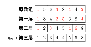
As shown in the figure, each level has an array that appears unordered. In fact, every number marked in red is to be assigned to the left child. What is the assignment rule? Compare it with the median of this level: if it is less than or equal to the median, assign it to the left; otherwise, assign it to the right. However, note that the rule is not strictly assign to the left if it is less than or equal, and to the right otherwise. The median may occur multiple times, and the rule is also related to whether $N$ is odd or even. The code below demonstrates a clever way to handle this; you can refer to the code.

We cannot sort every level each time, since even ignoring the constant factors, the theoretical complexity would be too high. To find the median, one sort is enough. Why? For example, the median of $l,r$ is simply num[mid] after sorting.

There are two key arrays:

tree[log(N),N]: the tree, which stores all values, with space complexity $O(n\log n)$. toleft[log(N),n]: the number of elements among 1~i at each level that enter the left child. This should be understood as a prefix sum.

procedure Build(left,right,deep:longint); // left,right denote the left and right endpoints of the interval, deep is the layer number
var
  i,mid,same,ls,rs,flag:longint; // flag is used to balance the counts on the two sides
begin
  if left=right then exit; // the bottom layer has been reached
  mid:=(left+right) >> 1;
  same:=mid-left+1;
  for i:=left to right do 
    if tree[deep,i]<num[mid] then
      dec(same);

  ls:=left; // pointer to the first element assigned to the left child
  rs:=mid+1; // pointer to the first element assigned to the right child
  for i:=left to right do
  begin
    flag:=0;
    if (tree[deep,i]<num[mid])or((tree[deep,i]=num[mid])and(same>0)) then // condition for assigning to the left
    begin
      flag:=1; tree[deep+1,ls]:=tree[deep,i]; inc(ls);
      if tree[deep,i]=num[mid] then // balance the counts on both sides
        dec(same);
    end
    else
    begin
      tree[deep+1,rs]:=tree[deep,i]; inc(rs);
    end;
    toleft[deep,i]:=toleft[deep,i-1]+flag;
  end;
  Build(left,mid,deep+1); // continue
  Build(mid+1,right,deep+1);
end;

Queries

Let us first briefly revisit chairman trees. When using a chairman tree to find the $K$-th smallest element in an interval, we use $K$ as the reference: go left when going left, and subtract the value going left when going right. The same applies to a partition tree.

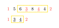
The difficult part of queries is shrinking the interval. In the figure below, the query is for $3$ through $7$, so at the next level we only need to query $2$ through $3$. Let $[\text{left},\text{right}]$ denote the shrunken interval (the target interval), while $[l,r]$ remains the interval of the current node. Why mark the target interval? Because it is the basis for deciding whether the answer lies on the left or the right.

function Query(left,right,k,l,r,deep:longint):longint;
var
  mid,x,y,cnt,rx,ry:longint;
begin
  if left=right then // writing l=r is also fine, because the target interval must contain an answer
    exit(tree[deep,left]);
  mid:=(l+r) >> 1;
  x:=toleft[deep,left-1]-toleft[deep,l-1]; // number going to the left child from l to left
  y:=toleft[deep,right]-toleft[deep,l-1]; // number going to the left child from l to right
  ry:=right-l-y; rx:=left-l-x; // ry is the number going to the right child from l to right, and rx is the number going to the right child from l to left
  cnt:=y-x; // number of left children from left to right
  if cnt>=k then // standard knowledge about chairman trees
    Query:=Query(l+x,l+y-1,k,l,mid,deep+1) // l+x is the shrunken left boundary, and l+y-1 is the shrunken right boundary; in the figure above, nodes 1 and 2 are discarded
  else
    Query:=Query(mid+rx+1,mid+ry+1,k-cnt,mid+1,r,deep+1); // this also shrinks the interval, but to the right; note that k must be reduced by cnt
end;

Properties

Time complexity: one query takes only $O(\log n)$, so $m$ queries take $O(m\log n)$.

Space complexity: only $O(n\log n)$ numbers need to be stored.

Measured results: chairman tree: $1482 \text{ms}$, partition tree: $889 \text{ms}$. (Non-recursive, with small constant factors.)

Applications of partition trees

Example problem: Luogu P3157[CQOI2011] Dynamic inversion pairs

Brief problem statement: Given a permutation of $n$ elements ($n\leq 10^5$), there are m queries ($m\leq 5\times 10^4$). Each time, delete one number from the permutation and find the number of inversion pairs remaining afterward.

This problem can be solved with CDQ in $\Theta(n\log^2n)$ time and $\Theta(n)$ space, and CDQ also has excellent constant factors.

If the problem is changed to require online processing, the usual solution is a segment tree of trees built from a Fenwick tree and a chairman tree, with time complexity $\Theta(n\log^2n)$ and space complexity $\Theta(n\log^2n)$. Its constant factor is somewhat larger, but it can also pass this problem.

Using a partition tree, this problem can be solved online in $\Theta(n\log^2n)$ time and $\Theta(n\log n)$ space, with a much smaller constant factor than the segment-tree-of-trees solution. (Roughly comparable to CDQ.)

For each node in a partition tree, we call it a right node if and only if it is divided into the right child at the next level, namely, if it is one of the elements appearing later in the original array; left nodes are defined similarly. If the top level is sorted while building the tree, then, similarly to counting inversion pairs with merge sort, the number of inversion pairs in an array is the sum of the numbers of right nodes before each left node.

Now consider deletion. Deleting a left node reduces the inversion count of the entire array by the number of right nodes before it, while deleting a right node reduces it by the number of left nodes after it. We can therefore dynamically maintain the “number of right nodes before each left node” and the “number of left nodes after each right node.” This can be maintained simply with a Fenwick tree.

Note that when using a Fenwick tree, we can only count contributions within the same block of the partition tree, not contributions that leave the block. There is a clever way to handle this with a Fenwick tree.

The index range of every block in a partition tree must have the form $[c\times 2^k+1,(c+1)\times 2^k]$. The blocks are listed below (because the code does not involve processing the bottom level of the partition tree, only the penultimate level is listed):

[0001 0010] [0011 0100] [0101 0110] [0111 1000] [1001 1010] [1011 1100] [1101 1110] [1111 10000]  lev=1
[0001 0010 0011 0100]   [0101 0110 0111 1000]   [1001 1010 1011 1100]   [1101 1110 1111 10000]    lev=2
[0001 0010 0011 0100 0101 0110 0111 1000]       [1001 1010 1011 1100 1101 1110 1111 10000]        lev=3
[0001 0010 0011 0100 0101 0110 0111 1000 1001 1010 1011 1100 1101 1110 1111 10000]                lev=4

Recall how a Fenwick tree works: when jumping upward, we perform x += lowbit(x) each time. If we ensure that upward jumps never leave the block, then only values inside the block are affected. Upward queries work similarly.

To ensure that an upward jump does not leave the block, we only need to require $lowbit(x)<2^{lev}$ at each jump.

Downward jumps are handled quite differently. If the index range of each block is written using 0-based indexing, it has the form $[c\times 2^k,(c+1)\times 2^k)$. Thus, shifting an index right by k bits is enough to determine which block it belongs to. When jumping downward, simply check continuously whether the jump leaves the block.

Note that the Fenwick tree implemented this way will access the largest power of 2 closest to n as its largest index, so the array index cannot be allocated as n.

Since we need to make updates on $\log n$ levels, and an update on level $k$ has time complexity $\Theta(k)$, the final time complexity is $\Theta(n\log n+m\log^2n)$.

Code:

#include <algorithm>
#include <cstring>
#include <iostream>
#if defined(_MSC_VER) && !defined(__clang__)
#include <immintrin.h>
#define __builtin_clz _lzcnt_u32
#endif
using namespace std;
using lld = long long;

int ti[2][17][131073];

int lowbit(int x) { return x & (-x); }

void fixup(int k, int x) {
  for (; lowbit(x) < 1 << k; x += lowbit(x)) {
    ++ti[0][k - 1][x];
  }
  ++ti[0][k - 1][x];
}

void fixdown(int k, int x) {
  for (; ((x ^ lowbit(x)) - 1) >> k == (x - 1) >> k; x ^= lowbit(x)) {
    ++ti[1][k - 1][x];
  }
  ++ti[1][k - 1][x];
}

int queryup(int k, int x) {
  int res = 0;
  for (; lowbit(x) < 1 << k; x += lowbit(x)) {
    res += ti[1][k - 1][x];
  }
  return res + ti[1][k - 1][x];
}

int querydown(int k, int x) {
  int res = 0;
  for (; ((x ^ lowbit(x)) - 1) >> k == (x - 1) >> k; x ^= lowbit(x)) {
    res += ti[0][k - 1][x];
  }
  return res + ti[0][k - 1][x];
}

int ai[100005];
int tx[100005];

lld mgx(int* npi, int* nai, int* rxi, int* lxi, int al, int ar, int bl,
        int br) {
  int rx = 1;
  int lx = ar - al;
  lld res = 0;
  for (; al != ar || bl != br; ++npi, ++nai, ++rxi, ++lxi) {
    if (al != ar && (bl == br || tx[al] < tx[bl])) {
      --lx;
      *rxi = rx;
      *nai = tx[al];
      *npi = al;
      ++al;
    } else {
      ++rx;
      *lxi = lx;
      res += ar - al;
      *nai = tx[bl];
      *npi = bl;
      ++bl;
    }
  }
  return res;
}

int npi[1700005];
int nri[1700005];
int nli[1700005];

int main() {
  cin.tie(nullptr)->sync_with_stdio(false);
  int n, m;
  cin >> n >> m;
  for (int i = 1; i <= n; ++i) cin >> ai[i];

  if (n == 1) {
    for (int i = 1; i <= m; ++i) cout << "0\n";
    return 0;
  }

  const int logn = 31 - __builtin_clz(n - 1);

  lld ans = 0;
  for (int i = logn; i >= 0; --i) {
    memcpy(tx, ai, (n + 1) * sizeof(int));
    for (int j = 1; j <= n; j += 1 << (logn - i + 1)) {
      ans += mgx(npi + n * i + j, ai + j, nri + n * i + j, nli + n * i + j, j,
                 min(n + 1, j + (1 << (logn - i))),
                 min(n + 1, j + (1 << (logn - i))),
                 min(n + 1, j + (1 << (logn - i + 1))));
    }
  }
  cout << ans << '\n';

  for (int asdf = 1; asdf < m; ++asdf) {
    int x;
    cin >> x;
    for (int i = 0, p = 0; i <= logn; ++i, p += n) {
      if (nri[p + x]) {
        ans -= nri[p + x] - querydown(logn - i + 1, x) - 1;
        fixdown(logn - i + 1, x);
      } else {
        ans -= nli[p + x] - queryup(logn - i + 1, x);
        fixup(logn - i + 1, x);
      }
      x = npi[p + x];
    }
    cout << ans << '\n';
  }
}

Afterword

Reference blog post: link.