AIOJ

This page briefly introduces how to use Splay to maintain a binary search tree.

Definition

A Splay tree, also called a self-adjusting tree, is a balanced binary search tree that repeatedly rotates a node to the root through splay operations. This preserves the binary-search-tree property, supports insertion, lookup, and deletion in amortized $O(\log N)$ time, and keeps the tree balanced instead of letting it degenerate into a chain.

Splay trees were invented by Daniel Sleator and Robert Tarjan in 1985.

Basic Structure and Operations

This section discusses the basic structure of a Splay tree and its core operations, the most important of which is the splay operation.

A Splay tree is a binary search tree. When searching for a value, it satisfies the property that every value in the left subtree is $<$ the root value, which is $<$ every value in the right subtree.

Maintained Information

This article uses arrays to simulate pointers when implementing a Splay tree. The following information must be maintained:

rt	id	fa[i]	ch[i][0/1]	val[i]	cnt[i]	sz[i]
Root node number	Number of used nodes	Parent	Left and right child numbers	Node value	Number of occurrences of the value	Subtree size

During initialization, it is sufficient to set all information to zero.

Helper Operations

First, here are some simple helper operations:

dir(x): determine whether node $x$ is the left or right child of its parent;
push_up(x): after a node changes position, update the information for node $x$ using the information from its children.

Implementation

bool dir(int x) { return x == ch[fa[x]][1]; }

void push_up(int x) { sz[x] = cnt[x] + sz[ch[x][0]] + sz[ch[x][1]]; }

Rotation

To keep a Splay tree balanced, we need rotation operations. A rotation moves a node one level upward.

A rotation must ensure that:

the in-order traversal of the entire Splay tree remains unchanged (so the binary-search-tree property is preserved);
the maintained information for all affected nodes remains correct;
rt points to the root after the rotation.

There are two kinds of rotations in a Splay tree: left rotation and right rotation.

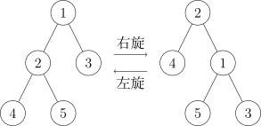
As the figure shows, when moving node $x$ upward by a rotation ( $1$ for a left rotation and $2$ for a right rotation), the direction of the rotation is determined uniquely by whether the node is the left or right child of its parent. Thus, when implementing rotation, it is enough to pass in the node $x$ to be moved upward.

Analyze the rotation step by step (assume that $x$ is the node to be moved upward, and use a right rotation as an example):

First record node $x$ and its parent $y$ , then record $y$ 's parent $z$ (which may be empty), and whether $x$ is the left or right child of $y$ ;
Following the bottom-up order in the rotated tree, update $y$ 's left child to be the right child of $x$ , $x$ 's right child to be $y$ , and, if $z$ is nonempty, the corresponding child of $z$ to be $x$ ;
In the same order, update the parent of the current left child of $y$ (if it exists) to $y$ , the parent of $y$ to $x$ , and the parent of $x$ to $z$ ;
Maintain the node information from bottom to top.

Implementation

void rotate(int x) {
  int y = fa[x], z = fa[y];
  bool r = dir(x);
  ch[y][r] = ch[x][!r];
  ch[x][!r] = y;
  if (z) ch[z][dir(y)] = x;
  if (ch[y][r]) fa[ch[y][r]] = y;
  fa[y] = x;
  fa[x] = z;
  push_up(y);
  push_up(x);
}

When implementing every function, be careful not to modify the information stored at node $0$ .

Splay Operation

A Splay tree requires every node $x$ to be rotated to the root immediately after it is accessed. This operation is called a splay operation.

Let $x$ be the node that was just accessed. A splay operation applies a sequence of splay steps to $x$ . Each splay step moves $x$ closer to the root, shortening the distance from $x$ to the root. Let $p$ be the parent of $x$ . There are three kinds of splay steps:

zig: Apply this when $p$ is the root. The Splay tree rotates according to the edge between $x$ and $p$ . zig exists to handle parity; it is used as the final step of a splay operation only when $x$ has odd depth at the start of the operation.

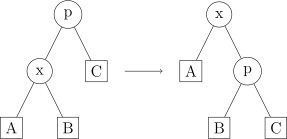
splay-zig

In other words, rotate $x$ directly to the right or left (Figures 1 and 2).

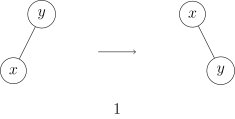
Figure 1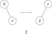
Figure 2
zig-zig: Apply this when $p$ is not the root and $x$ and $p$ are both right children or both left children. The figure below shows the case where both $x$ and $p$ are left children. The Splay tree first rotates across the edge connecting $p$ to its parent $g$ , then rotates across the edge connecting $x$ and $p$ .

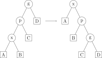
splay-zig-zig

That is, first rotate $p$ right or left, then rotate $x$ right or left (Figures 3 and 4).

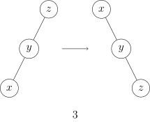
Figure 3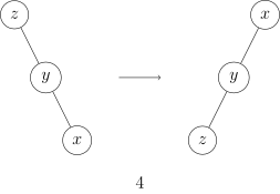
Figure 4
zig-zag: Apply this when $p$ is not the root and one of $x$ and $p$ is a right child while the other is a left child. The Splay tree first rotates across the edge between $p$ and $x$ , then rotates across the newly formed edge between $x$ and $g$ .

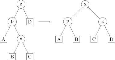
splay-zig-zag

That is, rotate $x$ left then right, or right then left (Figures 5 and 6).

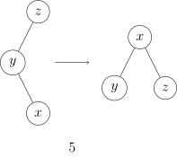
Figure 5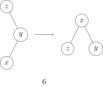
Figure 6

Tip

Try simulating the $6$ rotation cases yourself to understand the basic idea behind the splay operation.

Comparing the three splay steps, the key to choosing the correct operation is determining whether $x$ is a child of the root and whether $x$ and its parent are on the same side of their respective parents.

The implementation below can specify any root node $z$ and move any node $x$ in its subtree up to $z$ :

First record root node $z$ and its parent $w$ , so that fa[x] == w can be used to determine whether $x$ is already at the root position;
Record node $x$ 's current parent $y$ . If $y$ and $w$ are the same, $x$ has already reached the root;
Otherwise, use fa[y] == w to determine whether $y$ is the root. If it is, perform a zig operation directly to rotate $x$ ; otherwise, use dir(x) == dir(y) to choose between zig-zig and zig-zag. The former rotates $y$ first and then $x$ , while the latter rotates $x$ twice.

Implementation

void splay(int& z, int x) {
  int w = fa[z];
  for (int y; (y = fa[x]) != w; rotate(x)) {
    if (fa[y] != w) rotate(dir(x) == dir(y) ? y : x);
  }
  z = x;
}

The splay operation is the core operation of a Splay tree and the key step that guarantees its time complexity. Be sure to perform a splay operation after every downward access to a node.

In addition, a splay operation updates all node information on the path from the current node $x$ to the root $z$ in bottom-up order. This is why information at a non-root node can be modified first, then brought to the root by a splay operation to update the entire tree.

Time Complexity

The complexity for an $n$ -node Splay tree performing $m$ splay operations is $O((n+m)\log n)$ , so the amortized complexity of one operation is $O(\log n)$ .

Complexity Proof Based on Potential Analysis

We only need to analyze the complexity of the three operations zig, zig-zig, and zig-zag. We use potential analysis, deriving the amortized complexity by studying changes in potential. Suppose a Splay tree containing $n$ nodes undergoes $m$ splay operations. The analysis is as follows:

Definitions:

Potential of a single node: $w(x) = \log(\text{size}(x))$ , where $\text{size}(x)$ is the size of the subtree rooted at node $x$ .
Potential of the entire tree: $\varphi = \sum w(x)$ , the sum of the potentials of all nodes. Initially, $\varphi_0 \leq n \log n$ .
Amortized cost of the $i$ -th operation: $c_i = t_i + \varphi_i - \varphi_{i-1}$ , where $t_i$ is the actual cost, and $\varphi_i$ and $\varphi_{i-1}$ are the potentials after and before the operation.

Properties:

If $p$ is the parent of $x$ , then $w(p) \geq w(x)$ ; the potential of a parent is no smaller than that of its child.
Because the subtree size of the root remains unchanged before and after an operation, the potential of the root does not change during the operation.
If $\text{size}(p)\ge\text{size}(x)+\text{size}(y)$ , then $2w(p) - w(x) - w(y) \geq 2$ .

Proof of Property 3

By the arithmetic–geometric mean inequality,

\begin{aligned} 2w(p) - w(x) - w(y) &= \log\dfrac{\text{size}(p)^2}{\text{size}(x)\cdot\text{size}(y)} \\ &> \log\dfrac{\left(\text{size}(x)+\text{size}(y)\right)^2}{\text{size}(x)\cdot\text{size}(y)} \\ &\ge \log 4 \\ &= 2. \end{aligned}

Next, analyze the potential changes for zig, zig-zig, and zig-zag separately. The node notation is the same as in the previous section. Let the potentials of node $x$ before and after the operation be $w(x)$ and $w'(x)$ , respectively.

zig: By Properties 1 and 2, $w(p) = w'(x)$ and $w'(x) \geq w'(p)$ . Therefore, the amortized cost is

\begin{aligned} c_i &= 1 + w'(x) + w'(p) - w(x) - w(p)\\ &= 1 + w'(p) - w(x)\\ &\leq 1 + w'(x) - w(x). \end{aligned}

zig-zig: By Properties 1 and 2, $w(g) = w'(x)$ , $w'(x) \geq w'(p)$ , and $w(x) \leq w(p)$ . Because

\begin{aligned} \text{size}'(x) &= 3 + \text{size}(A) + \text{size}(B) + \text{size}(C) + \text{size}(D) \\ &> (1 + \text{size}(A) + \text{size}(B)) + (1 + \text{size}(C) + \text{size}(D)) \\ &= \text{size}(x) + \text{size}'(g), \end{aligned}

By Property 3,

2 w'(x) - w(x) - w'(g) \geq 2.

Therefore, the amortized cost is

\begin{aligned} c_i &= 2 + w'(x) + w'(p) + w'(g) - w(x) - w(p) - w(g) \\ &= 2 + w'(p) + w'(g) - w(x) - w(p) \\ &\le (2 w'(x) - w(x) - w'(g)) + w'(p) + w'(g) - w(x) - w(p) \\ &= 2(w'(x)-w(x)) + w'(p) - w(p) \\ &\le 3(w'(x)-w(x)). \end{aligned}

zig-zag: By Properties 1 and 2, $w(g) = w'(x)$ and $w(p) \geq w(x)$ . Because $\text{size}'(x)>\text{size}'(p)+\text{size}'(g)$ , Property 3 gives

2 \cdot w'(x) - w'(g) - w'(p) \geq 2.

Therefore, the amortized cost is

\begin{aligned} c_i &= 2 + w'(x) + w'(p) + w'(g) - w(x) - w(p) - w(g) \\ &= 2 + w'(p) + w'(g) - w(x) - w(p) \\ &\le (2w'(x) - w'(g) - w'(p)) + w'(p) + w'(g) - w(x) - w(p) \\ &= 2w'(x) - w(x) - w(p) \\ &\le 2(w'(x) - w(x)). \end{aligned}

A single splay operation:

Let $w^{(n)}(x)=(w^{(n-1)})'(x)$ and $w^{(0)}(x)=w(x)$ . Suppose one splay operation visits the nodes $x_{1}, x_{2}, \cdots, x_{n}$ in sequence, and $x_{1}$ finally becomes the root. This necessarily consists of several zig-zig and zig-zag operations and at most one zig operation. The amortized cost of each of the first two kinds of operations is at most $3(w'(x)-w(x))$ , and the amortized cost of the final operation is at most $3(w'(x) - w(x))+1$ , so the total amortized cost is at most

3(w^{(n)}(x_1) - w^{(0)}(x_1)) + 1 \le 3\log n + 1.

Therefore, the amortized complexity of a single splay operation is $O(\log n)$ . Consequently, insertion, lookup, deletion, and similar operations based on splaying also have amortized time complexity $O(\log n)$ .

Conclusion:

After $m$ splay operations, the actual cost is

\begin{aligned} \sum_{i=1}^m t_i &= \sum_{i=1}^m \left(c_i + \varphi_{i-1} - \varphi_i \right) \\ &= \sum_{i=1}^m c_i + \varphi_0 - \varphi_m \\ &\le m(3\log n+1) + n\log n. \end{aligned}

Therefore, the actual time complexity of $m$ splay operations is $O((m+n)\log n)$ .

Why Does Rebalancing a Splay Tree Have Amortized Complexity

O(\log n)

The naive rebalancing idea is to repeatedly rotate a node upward until it becomes the root. For a chain-shaped tree in which all child nodes are left (or right) children, this is equivalent to repeatedly performing zig operations. The constant term $1$ in the amortized complexity of zig then accumulates, ultimately making the amortized complexity $O(\log n+n)$ . The design of Splay tree rebalancing avoids this accumulation of the constant term in a sequence of consecutive zig operations: a complete splay operation performs at most one standalone zig operation, which improves the time complexity.

Balanced-Tree Operations

This section discusses common operations for implementing a balanced tree with a Splay tree. Of particular importance are finding an element by value or by rank: these operations locate a specific element and move it to the root for subsequent processing.

As an example, this section discusses the implementation of the template problem Ordinary Balanced Tree.

Finding by Value

As a binary search tree, a Splay tree can find the node corresponding to a value $v$ by comparing the target value $v$ with the value of the current node. Once the node is found, move it to the root.

The corresponding node may not exist in the tree. In this case, record the last accessed node (the $y$ in the implementation) and move $y$ to the root. The value stored at $y$ must then be either the largest value among all values smaller than $v$ (the predecessor of $v$ ), or the smallest value among all values larger than $v$ (the successor of $v$ ). This follows because the search process keeps values smaller than $v$ in the left subtree and values larger than $v$ in the right subtree.

Implementation

void find(int& z, int v) {
  int x = z, y = fa[x];
  for (; x && val[x] != v; x = ch[y = x][v > val[x]]);
  splay(z, x ? x : y);
}

This implementation allows any node $z$ to be specified as the root, and searches by value within its subtree.

Accessing by Rank

Because subtree sizes are maintained, a Splay tree can also access an element by rank, that is, find the $k$ -th smallest element in the tree.

Let $k$ be the remaining rank. The procedure is:

If the left subtree is nonempty and the remaining rank $k$ is no greater than its size, search in the left subtree;
Otherwise, if $k$ is no greater than the size of the left subtree plus the size of the root's multiplicity, the root is the element being sought;
Otherwise, subtract the sizes of the left subtree and the root's multiplicity from $k$ , and continue searching in the right subtree;
Move the element eventually found to the root.

Implementation

void loc(int& z, int k) {
  int x = z;
  for (;;) {
    if (sz[ch[x][0]] >= k) {
      x = ch[x][0];
    } else if (sz[ch[x][0]] + cnt[x] >= k) {
      break;
    } else {
      k -= sz[ch[x][0]] + cnt[x];
      x = ch[x][1];
    }
  }
  splay(z, x);
}

This implementation requires that rank $k$ not exceed the tree size at root $z$ .

In the template problem, operation $4$ asks for the value at a given rank. It can directly call this method and return the value.

Implementation

int find_kth(int k) {
  if (k > sz[rt]) return -1;
  loc(rt, k);
  return val[rt];
}

Merging

Sometimes two Splay trees need to be merged.

Let the roots of the two trees be $x$ and $y$ . To ensure that the result is still a binary search tree, every value in the $x$ tree must be smaller than every value in the $y$ tree. This condition can usually be met because the two trees are often split from a larger subtree.

The merge operation is as follows:

If either $x$ or $y$ , or both, are empty trees, directly return the root of the nonempty tree, or an empty tree;
Otherwise, use loc(y, 1) to move the minimum value in the $y$ tree to its root $y$ , then set its left child (which must now be empty) to $x$ , update the node information, and return $y$ .

Implementation

int merge(int x, int y) {
  if (!x || !y) return x | y;
  loc(y, 1);
  ch[y][0] = x;
  fa[x] = y;
  push_up(y);
  return y;
}

Splitting is similar. Thus, a Splay tree can imitate the approach of a non-rotating treap to perform various operations, including interval operations. The later section introduces an interval-operation method that is more characteristic of Splay trees.

Insertion

Insertion is a relatively complicated process. The steps are as follows (assume that the inserted value is $v$ ):

As in a search by value, search downward according to $v$ until reaching the node storing $v$ or an empty node, recording the parent node $y$ along the way;
If a node storing $v$ exists, namely node $x$ , update its information directly; otherwise create a new node $x$ ;
Perform a splay operation to move the final node $x$ to the root.

Implementation

void insert(int v) {
  int x = rt, y = 0;
  for (; x && val[x] != v; x = ch[y = x][v > val[x]]);
  if (x) {
    ++cnt[x];
    ++sz[x];
  } else {
    x = ++id;
    val[x] = v;
    cnt[x] = sz[x] = 1;
    fa[x] = y;
    if (y) ch[y][v > val[y]] = x;
  }
  splay(rt, x);
}

This implementation can insert a value directly into an empty tree. If you do not want to handle an empty tree, insert a dummy node into the tree in advance.

Deletion

Deletion is also a relatively complicated process. The steps are as follows (assume that the value being deleted is $v$ ):

First search for the node storing $v$ by value and move it to the root;
If no node storing it exists, return directly (the preceding step has already performed the splay operation);
Otherwise, update the node information;
If the resulting root is an empty node, merge the left and right subtrees as the new root. Before merging, remember to set the parent of each subtree root to empty.

Implementation

bool remove(int v) {
  find(rt, v);
  if (!rt || val[rt] != v) return false;
  --cnt[rt];
  --sz[rt];
  if (!cnt[rt]) {
    int x = ch[rt][0];
    int y = ch[rt][1];
    fa[x] = fa[y] = 0;
    rt = merge(x, y);
  }
  return true;
}

Querying the Rank

Access node $v$ by value (and move it to the root), then return the corresponding value directly.

When $v$ does not exist, the relationship between the returned root and $v$ is not determined by find(rt, v), so it must be handled separately.

Implementation

int find_rank(int v) {
  find(rt, v);
  return sz[ch[rt][0]] + (val[rt] < v ? cnt[rt] : 0) + 1;
}

Querying the Predecessor

The predecessor is the largest value smaller than $v$ . The procedure is:

Access node $v$ by value (and move it to the root);
If the root value is smaller than $v$ , it must be the largest such value, so return it directly;
Otherwise, find the maximum value in the left subtree and move it to the root.

The last step is equivalent to directly calling loc(ch[rt][0], sz[ch[rt][0]]), with unnecessary checks omitted.

Implementation

int find_prev(int v) {
  find(rt, v);
  if (rt && val[rt] < v) return val[rt];
  int x = ch[rt][0];
  if (!x) return -1;
  for (; ch[x][1]; x = ch[x][1]);
  splay(rt, x);
  return val[rt];
}

This implementation allows the predecessor not to exist; in that case it returns $-1$ .

Querying the Successor

The successor is the smallest value greater than $x$ . The query method is similar to that for the predecessor, except that it replaces the maximum value in the left subtree with the minimum value in the right subtree, namely, it calls loc(ch[rt][1], 1).

Implementation

int find_next(int v) {
  find(rt, v);
  if (rt && val[rt] > v) return val[rt];
  int x = ch[rt][1];
  if (!x) return -1;
  for (; ch[x][0]; x = ch[x][0]);
  splay(rt, x);
  return val[rt];
}

Reference Implementation

Finally, this section gives the reference implementation for the template problem Ordinary Balanced Tree.

Reference implementation

#include <iostream>

constexpr int N = 2e6;
int id, rt;
int fa[N], val[N], cnt[N], sz[N], ch[N][2];

// --8<-- [start:aux]
bool dir(int x) { return x == ch[fa[x]][1]; }

void push_up(int x) { sz[x] = cnt[x] + sz[ch[x][0]] + sz[ch[x][1]]; }

// --8<-- [end:aux]
// --8<-- [start:rotate]
void rotate(int x) {
  int y = fa[x], z = fa[y];
  bool r = dir(x);
  ch[y][r] = ch[x][!r];
  ch[x][!r] = y;
  if (z) ch[z][dir(y)] = x;
  if (ch[y][r]) fa[ch[y][r]] = y;
  fa[y] = x;
  fa[x] = z;
  push_up(y);
  push_up(x);
}

// --8<-- [end:rotate]
// --8<-- [start:splay]
void splay(int& z, int x) {
  int w = fa[z];
  for (int y; (y = fa[x]) != w; rotate(x)) {
    if (fa[y] != w) rotate(dir(x) == dir(y) ? y : x);
  }
  z = x;
}

// --8<-- [end:splay]
// --8<-- [start:find]
void find(int& z, int v) {
  int x = z, y = fa[x];
  for (; x && val[x] != v; x = ch[y = x][v > val[x]]);
  splay(z, x ? x : y);
}

// --8<-- [end:find]
// --8<-- [start:loc]
void loc(int& z, int k) {
  int x = z;
  for (;;) {
    if (sz[ch[x][0]] >= k) {
      x = ch[x][0];
    } else if (sz[ch[x][0]] + cnt[x] >= k) {
      break;
    } else {
      k -= sz[ch[x][0]] + cnt[x];
      x = ch[x][1];
    }
  }
  splay(z, x);
}

// --8<-- [end:loc]
// --8<-- [start:merge]
int merge(int x, int y) {
  if (!x || !y) return x | y;
  loc(y, 1);
  ch[y][0] = x;
  fa[x] = y;
  push_up(y);
  return y;
}

// --8<-- [end:merge]
// --8<-- [start:insert]
void insert(int v) {
  int x = rt, y = 0;
  for (; x && val[x] != v; x = ch[y = x][v > val[x]]);
  if (x) {
    ++cnt[x];
    ++sz[x];
  } else {
    x = ++id;
    val[x] = v;
    cnt[x] = sz[x] = 1;
    fa[x] = y;
    if (y) ch[y][v > val[y]] = x;
  }
  splay(rt, x);
}

// --8<-- [end:insert]
// --8<-- [start:remove]
bool remove(int v) {
  find(rt, v);
  if (!rt || val[rt] != v) return false;
  --cnt[rt];
  --sz[rt];
  if (!cnt[rt]) {
    int x = ch[rt][0];
    int y = ch[rt][1];
    fa[x] = fa[y] = 0;
    rt = merge(x, y);
  }
  return true;
}

// --8<-- [end:remove]
// --8<-- [start:find-rank]
int find_rank(int v) {
  find(rt, v);
  return sz[ch[rt][0]] + (val[rt] < v ? cnt[rt] : 0) + 1;
}

// --8<-- [end:find-rank]
// --8<-- [start:find-kth]
int find_kth(int k) {
  if (k > sz[rt]) return -1;
  loc(rt, k);
  return val[rt];
}

// --8<-- [end:find-kth]
// --8<-- [start:find-prev]
int find_prev(int v) {
  find(rt, v);
  if (rt && val[rt] < v) return val[rt];
  int x = ch[rt][0];
  if (!x) return -1;
  for (; ch[x][1]; x = ch[x][1]);
  splay(rt, x);
  return val[rt];
}

// --8<-- [end:find-prev]
// --8<-- [start:find-next]
int find_next(int v) {
  find(rt, v);
  if (rt && val[rt] > v) return val[rt];
  int x = ch[rt][1];
  if (!x) return -1;
  for (; ch[x][0]; x = ch[x][0]);
  splay(rt, x);
  return val[rt];
}

// --8<-- [end:find-next]
int main() {
  int n;
  std::cin >> n;
  for (; n; --n) {
    int op, x;
    std::cin >> op >> x;
    switch (op) {
      case 1:
        insert(x);
        break;
      case 2:
        remove(x);
        break;
      case 3:
        std::cout << find_rank(x) << '\n';
        break;
      case 4:
        std::cout << find_kth(x) << '\n';
        break;
      case 5:
        std::cout << find_prev(x) << '\n';
        break;
      case 6:
        std::cout << find_next(x) << '\n';
        break;
    }
  }
  return 0;
}

Sequence Operations

A Splay tree can also be used on a sequence to maintain interval information. Compared with a segment tree, a Splay tree has larger constants but supports more complex sequence operations, such as interval reversal. As mentioned above, Splay trees also support splitting and merging, so they can imitate a non-rotating treap for interval operations; this will not be discussed further here. This section focuses on implementing interval operations based on splay operations.

A Splay tree built from a sequence has the following properties:

The in-order traversal of the Splay tree is equivalent to traversing the original sequence from left to right;
Each node in the Splay tree represents one element of the original sequence;
A subtree of the Splay tree represents an interval of the original sequence.

Because splay operations are available, the Splay subtree representing an interval can be extracted quickly.

As an example, this section discusses the implementation of the template problem Artistic Balanced Tree.

Building the Tree from a Sequence

Before performing operations, build the Splay tree from the given sequence. By the properties of a Splay tree, it is enough to build a chain in which every node is a left child. This takes $O(n)$ time.

Reference implementation

void build(int n) {
  for (int i = 1; i <= n + 2; ++i) {
    ++id;
    ch[id][0] = rt;
    if (rt) fa[rt] = id;
    rt = id;
    val[id] = i - 1;
  }
  splay(rt, 1);
}

The final splay operation updates the node information from bottom to top. To simplify the interval operations below, two sentinel nodes are added to the left and right ends of the sequence.

Interval Reversal

Take interval reversal as an example to understand how interval operations work (let the interval be $[L,R]$ ):

First move node $L-1$ to the root. Then, in its right subtree, move node $R+1$ to the root of that right subtree;
Now let $x$ be the left child of the right child of the root. The subtree rooted at $x$ represents the interval $[L,R]$ ;
At $x$ , perform the operation on interval $[L,R]$ and attach a lazy tag;
Push the tag down once at $x$ , then use a splay operation to move $x$ to the root.

The operation needed in the first step is the rank-access operation described in the balanced-tree section above, because the element's label is its rank. Its implementation differs slightly because lazy-tag management is involved.

Reference implementation

void reverse(int l, int r) {
  loc(rt, l);
  loc(ch[rt][1], r - l + 2);
  int x = ch[ch[rt][1]][0];
  lazy_reverse(x);
  push_down(x);
  splay(rt, x);
}

The final splay operation is not needed to preserve the complexity guarantee; it updates the node information. Because splaying involves the left and right children of node $x$ , the tag at $x$ must be pushed down once first. For interval reversal specifically, reversing a subinterval does not affect its ancestor nodes, so omitting this step is also correct. The implementation keeps these two lines to illustrate the general method.

Lazy-Tag Management

First, we need the helper functions lazy_reverse(x) and push_down(x). The former swaps the left and right children and updates the lazy tag; the latter pushes the tag downward.

Reference implementation

void lazy_reverse(int x) {
  std::swap(ch[x][0], ch[x][1]);
  lz[x] ^= 1;
}

void push_down(int x) {
  if (lz[x]) {
    if (ch[x][0]) lazy_reverse(ch[x][0]);
    if (ch[x][1]) lazy_reverse(ch[x][1]);
    lz[x] = 0;
  }
}

Then, simply push tags down whenever moving downward through a node. The template problem has relatively simple requirements: only the rank-search operation (namely loc) accesses nodes downward. Be sure to push down the tag before the function visits each new node.

Reference implementation

void loc(int& z, int k) {
  int x = z;
  for (push_down(x); sz[ch[x][0]] != k - 1; push_down(x)) {
    if (sz[ch[x][0]] >= k) {
      x = ch[x][0];
    } else {
      k -= sz[ch[x][0]] + 1;
      x = ch[x][1];
    }
  }
  splay(z, x);
}

Because all lazy tags on the traversed path have been removed while moving downward, no lazy tags need to be handled when the splay operation moves the node upward. However, handle the node selected for the interval operation carefully: it also lies on the splay path, but may have an unpushed tag immediately after the operation, so the tag must be pushed down before splaying, just as above.

Reference Implementation

Finally, this section gives the reference implementation for the template problem Artistic Balanced Tree.

Reference implementation

#include <iostream>

constexpr int N = 2e6;
int id, rt;
int fa[N], val[N], sz[N], lz[N], ch[N][2];

bool dir(int x) { return x == ch[fa[x]][1]; }

void push_up(int x) { sz[x] = 1 + sz[ch[x][0]] + sz[ch[x][1]]; }

// --8<-- [start:push-down]
void lazy_reverse(int x) {
  std::swap(ch[x][0], ch[x][1]);
  lz[x] ^= 1;
}

void push_down(int x) {
  if (lz[x]) {
    if (ch[x][0]) lazy_reverse(ch[x][0]);
    if (ch[x][1]) lazy_reverse(ch[x][1]);
    lz[x] = 0;
  }
}

// --8<-- [end:push-down]
void rotate(int x) {
  int y = fa[x], z = fa[y];
  bool r = dir(x);
  ch[y][r] = ch[x][!r];
  ch[x][!r] = y;
  if (z) ch[z][dir(y)] = x;
  if (ch[y][r]) fa[ch[y][r]] = y;
  fa[y] = x;
  fa[x] = z;
  push_up(y);
  push_up(x);
}

void splay(int& z, int x) {
  int w = fa[z];
  for (int y; (y = fa[x]) != w; rotate(x)) {
    if (fa[y] != w) rotate(dir(x) == dir(y) ? y : x);
  }
  z = x;
}

// --8<-- [start:push-down-lazy]
void loc(int& z, int k) {
  int x = z;
  for (push_down(x); sz[ch[x][0]] != k - 1; push_down(x)) {
    if (sz[ch[x][0]] >= k) {
      x = ch[x][0];
    } else {
      k -= sz[ch[x][0]] + 1;
      x = ch[x][1];
    }
  }
  splay(z, x);
}

// --8<-- [end:push-down-lazy]
// --8<-- [start:build]
void build(int n) {
  for (int i = 1; i <= n + 2; ++i) {
    ++id;
    ch[id][0] = rt;
    if (rt) fa[rt] = id;
    rt = id;
    val[id] = i - 1;
  }
  splay(rt, 1);
}

// --8<-- [end:build]
// --8<-- [start:reverse]
void reverse(int l, int r) {
  loc(rt, l);
  loc(ch[rt][1], r - l + 2);
  int x = ch[ch[rt][1]][0];
  lazy_reverse(x);
  push_down(x);
  splay(rt, x);
}

// --8<-- [end:reverse]
void print(int x) {
  if (!x) return;
  push_down(x);
  print(ch[x][0]);
  std::cout << val[x] << ' ';
  print(ch[x][1]);
}

void print() {
  loc(rt, 1);
  loc(ch[rt][1], sz[rt] - 1);
  print(ch[ch[rt][1]][0]);
}

int main() {
  int n, m;
  std::cin >> n >> m;
  build(n);
  for (; m; --m) {
    int l, r;
    std::cin >> l >> r;
    reverse(l, r);
  }
  print();
  return 0;
}

Exercises

All of the following problems use a bare Splay tree to maintain a binary search tree:

Splay trees also appear in more complex applications:

References and Notes

Some content in this article is adapted from the Algocode algorithm blog; special thanks to its authors!