Self-Adjusting Top Tree

author:F7487

Self-Adjusting Top Tree

Introduction

Self-Adjusting Top Tree is a data structure for maintaining a fully dynamic forest based on Top Tree theory, proposed by Tarjan and Werneck in their 2005 paper Self-Adjusting Top Trees. It is abbreviated as SATT.

Self-Adjusting Top Tree supports path updates/queries, subtree updates/queries, and non-local searches on any tree in a forest.

Splay Tree is the foundation of SATT, but the Splay Tree used by SATT differs from an ordinary Splay in some details (with several extensions).

Problem statement

Maintain a forest supporting the following operations:

• Delete or add an edge, while ensuring that the result remains a forest.

• Modify the weight of a simple path in a tree.

• Modify the weight of a subtree rooted at a given vertex.

• Query the sum of the weights on a simple path in a tree.

• Query the sum of the weights in a subtree rooted at a given vertex.

Tree contraction

For any tree, we can use the theory of tree contraction to contract it into a single edge.

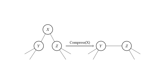
Specifically, tree contraction has two basic operations: Compress and Rake. A Compress operation selects a vertex $x$ of degree $2$, and denotes the two vertices adjacent to $x$ by $y$ and $z$. We add a new edge $yz$, store the information of vertex $x$ and edges $xz$ and $xy$ in $yz$, and delete them, as shown in the figure.

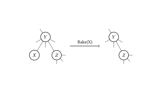
A Rake operation selects a vertex $x$ of degree $1$, and requires the degree of the vertex $y$ adjacent to $x$ to be greater than $1$. Let $z$ be the other neighbor of $y$. We store the information of vertex $x$ and edge $xy$ in edge $yz$, and delete them, as shown in the figure.

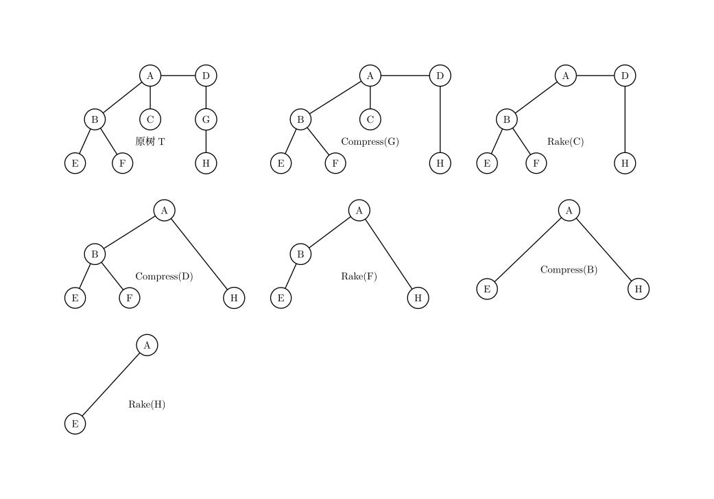
It is not difficult to prove that any tree can be contracted into a single edge using only Compress and Rake operations, as shown in the figure.

Clusters

For convenience, let the original tree before any operation be $T$. After applying some tree-contraction operations to $T$ (possibly none), let the resulting tree be $T_x$.

We study the information contained in an edge of some $T_x$.

Besides its own information (if the edge does not exist in $T$, it has no information of its own), this edge may also contain information about other vertices and edges merged into it through Compress/Rake operations. Let us first select an edge from the tree-contraction process in the figure below and see which vertices and edges it represents in $T$.

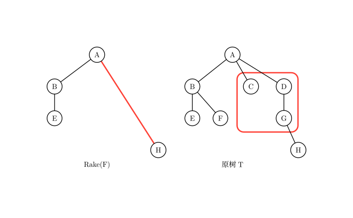
As shown in the figure, the selected edge and its corresponding graph are circled in red.

It can be seen that the vertices and edges represented in $T$ by the information contained in this edge are connected. We can generalize this: the information stored in any edge of any $T_x$ always forms a connected subgraph in $T$. We call such a connected subgraph a cluster.

However, a cluster is an incomplete subgraph: some endpoints of the edges it contains are not themselves included in the cluster. We call these endpoints the cluster's endpoints, the vertices of the connected subgraph that it contains internal nodes, and the edges of the connected subgraph internal edges.

Every cluster has the following properties:

1. A cluster stores and maintains only the information of its internal nodes and internal edges.

2. A cluster has two endpoints. These are exactly the two vertices joined by the edge in $T_x$ that represents the cluster. We call the path between the two endpoints the cluster path. If the two endpoints of a cluster are $x$ and $y$, we denote the cluster by $C(x,y)$.

3. An internal node is adjacent only to endpoints or internal nodes.

In particular, every edge in $T$ independently forms a cluster (containing only its own information); we call such a cluster a base cluster. In the final $T_x$, after $T$ has been contracted to a single edge, that edge represents a cluster containing all information of $T$ except for its two endpoints; we call this cluster the root cluster.

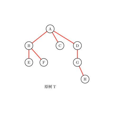
As shown in the figure, the base clusters mentioned above are marked with red lines.

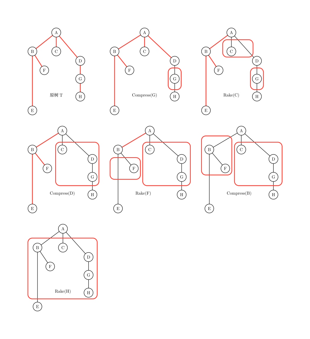
From the perspective of clusters, we see that Compress and Rake operations “merge two clusters into one”, leaving one new cluster. Thus, the tree-contraction process is also the process of merging all base clusters into one cluster.

Therefore, we can also obtain the following figure, which is another representation of a sequence of tree-contraction operations.

Top Tree

We now want to represent the entire process of contracting a tree.

We could use either of the two methods described above to represent this process, but that would be cumbersome: if tree contraction takes $n$ steps, we would need $n$ trees to represent the entire contraction.

Consider a simpler representation of a tree-contraction process on a tree. We introduce the Top Tree.

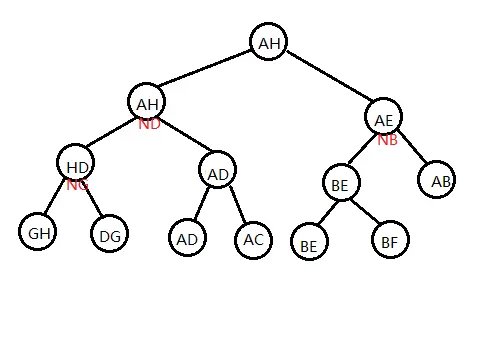
As shown in the figure, this is a Top Tree based on the contraction method and original tree described above.

A Top Tree has the following properties:

1. A Top Tree corresponds to an original tree and a way of contracting it. Every node of a Top Tree represents an edge in some $T_x$, that is, a cluster formed during tree contraction. A node shaped like $N_x$ in the figure represents the cluster formed by the compress(x) operation.

2. A node in a Top Tree has two children (each representing a cluster). The cluster represented by this node is the new cluster obtained by merging those two clusters through a Compress or Rake operation.

3. The leaf nodes of a Top Tree are base clusters, and its root node is the root cluster. Therefore, if we layer a Top Tree by topological order, each layer represents a $T_x$.

Maintaining information with a ternarized Self-Adjusting Top Tree

Principle

The substantial simplification of the tree-contraction process provided by a Top Tree reveals the possibility of maintaining information on a tree by maintaining that process. SATT maintains information on a tree according to this principle.

Notice that the tree-contraction process is also a process in which information on the tree is continuously added. When we perform compress(x), the information of vertex $x$ begins to appear in some cluster from that moment onward, affecting our aggregate results.

Suppose we now use a Top Tree to maintain a tree $T$, in which every vertex and edge has a weight, and we need to maintain the sum of the weights of $T$.

Now suppose we modify the weight of a vertex $x$ in $T$. Obviously, we need to update the information of every cluster in the Top Tree whose stored information contains $x$, giving a time complexity of $O(n)$ for a single operation.

However, if we choose a vertex for which the number of nodes in the Top Tree whose cluster information contains $x$ is small—in other words, if its information is added to clusters as late as possible—the time complexity of a single operation is greatly improved, as shown in the figure.

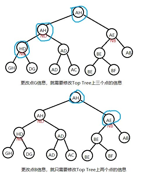
SATT maintains information on a tree by changing the order in which the information of a vertex/a path is added to clusters during tree contraction (to reduce the time complexity of a single operation when that vertex or path is modified).

Actual structure

We first root an original tree $T$ by depth, and then consider the root cluster of a Top Tree for some tree-contraction order. It has two endpoints; we let one of them be the root of the original tree, and choose the other endpoint arbitrarily.

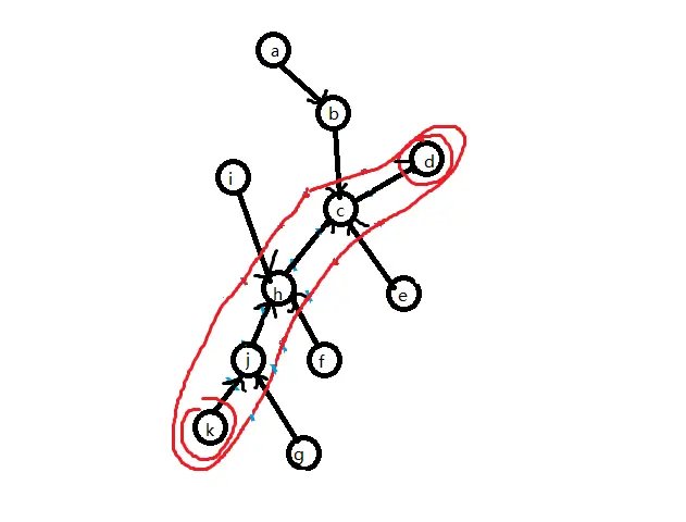
As shown in the figure, a pair of endpoints is selected for the root cluster; when marking the cluster here, the endpoints are circled as well.

From the basic operations of tree contraction, we know that the information of the vertices and edges $(j,h,c,jh,hc)$ on the cluster path is ultimately added to $C(k,g)$ through Compress operations, while the information of the non-cluster-path vertices $(a,b,i,f,g,e,ig,\cdots)$ is added to $C(k,g)$ through Rake operations.

We isolate the cluster path. It is a tree with a special shape (a path), and we build a Top Tree for this tree (with an arbitrary tree-contraction order).

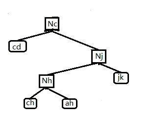
We call this structure a Compress Tree, because in this Top Tree, the two children of any node are merged into their parent through a Compress operation.

The nodes in a Compress Tree are called Compress Nodes. Considering only the current cluster path, a non-leaf Compress Node represents one compress process: it merges the information of its left and right children, then adds the information of vertex $x$ stored by compress(x) itself. This Compress Tree maintains the information of the cluster path of $C(k,g)$.

In addition, we impose some restrictions on the Top Tree used in the Compress Tree. Notice that the Compress Tree maintains a path of vertices in $T$ whose depths are pairwise distinct. We require the in-order traversal of the base clusters in the Compress Tree to have the same order as the depths of the corresponding edges in $T$, with a smaller in-order position corresponding to a shallower depth. Likewise, the relations represented by compress(x) for each vertex $x$ follow the same rule.

Now consider the information on the non-cluster paths. Suppose that the vertices and edges on these non-cluster paths have already formed a collection of maximal clusters, and that these maximal clusters were formed by Rake operations among the smaller clusters circled in blue. We represent the process of merging some smaller clusters into a maximal cluster with a ternary tree. Similarly, we call this structure a Rake Tree, and its nodes are called Rake Nodes. Every Rake Node represents a cluster formed by Raking the clusters represented by its left and right children into the cluster represented by its middle child. As shown below, every node in a Rake Tree represents a smaller cluster in $T$ with the same endpoints.

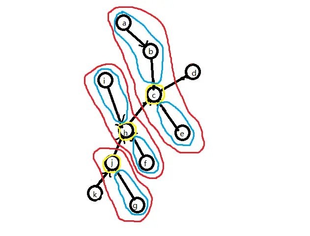
As shown in the figure, the clusters circled in blue are maximal clusters, and those circled in yellow are smaller clusters.

We process those smaller clusters in the same way: select their cluster paths, build Compress Trees, and so on recursively. In this way, we build many Compress Trees and Rake Trees representing the tree-contraction process.

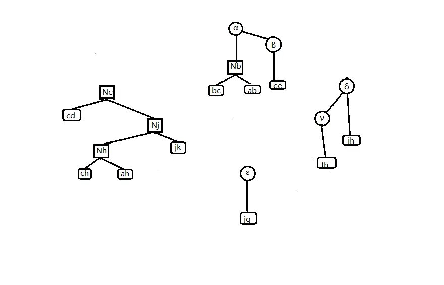
The figure above shows the Rake-Compress Tree of the original tree (because each Rake Node is connected to a Compress Tree, it appears as a Rake Tree connected to many Compress Trees) and the Compress Tree representing the root-cluster path.

Consider joining these trees together in some way so that they form an ordered whole. Let the common endpoint of the set of minimal clusters represented by a Rake Tree be $x$. We add the other, non-$x$ endpoint to the middle child (a collection of Compress Trees) of each of these Rake Nodes, while preserving the in-order traversal and the basic properties of the Top Tree, as shown in the figure.

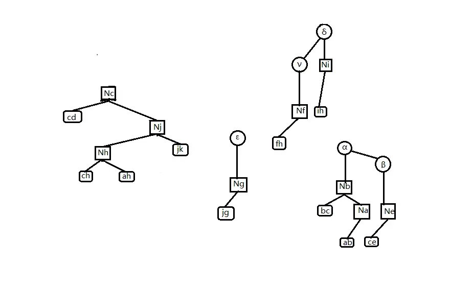
This step is equivalent to making the operation of adding a vertex of $T$ by a Rake operation occur directly in the Compress Tree. This not only lets us maintain the information of Rake Nodes correctly (by simply merging the information of their three children), but also makes the structure of our Compress Tree more complete. Next, we ternarize the Compress Tree: if the common endpoint of a Rake Tree is $x$, we attach the Rake Tree to the middle child of compress(x), as shown in the figure.

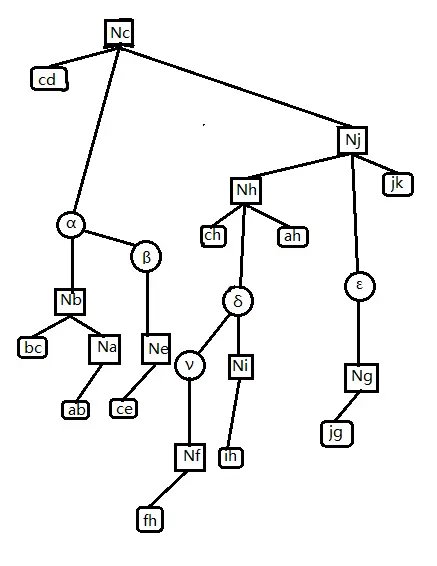
After ternarization, the meaning of the compress(x) node becomes: first Rake its middle child into the cluster path, then aggregate the information of its left and right children and vertex $x$.

Finally, we process the Compress Tree of the root-cluster path in the same way as every other Compress Tree: insert its two endpoints according to the in-order traversal, so that its root stores the information of the entire $T$.

Thus, we implement information maintenance on a tree using a ternarized Self-Adjusting Top Tree.

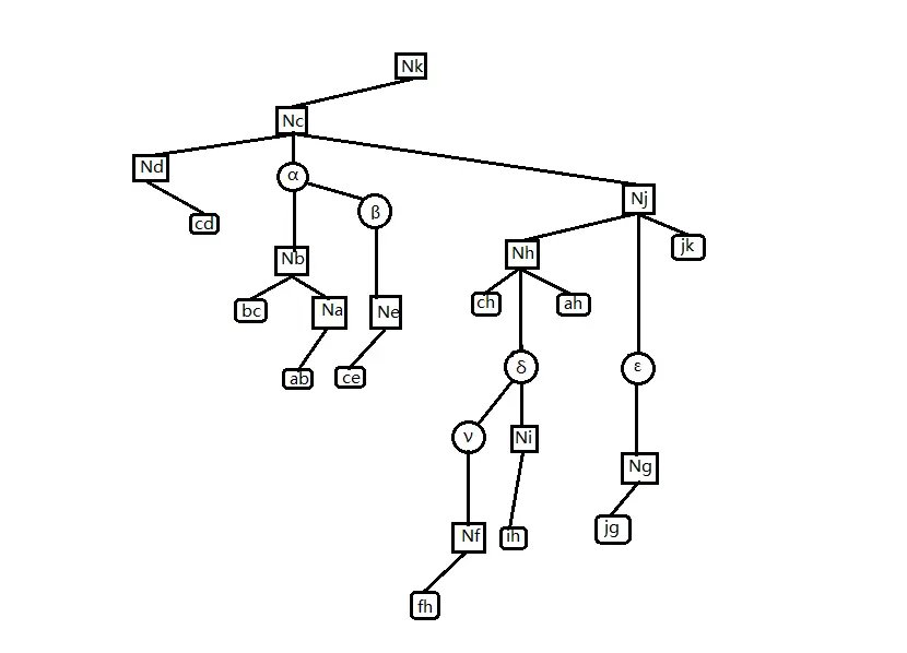
In summary, SATT has the following properties:

1. SATT consists of Compress Trees and Rake Trees. A Compress Tree is a special Top Tree; a Rake Tree is a ternary tree. Both correspond to the process of contracting a tree.

2. A node in a Compress Tree has at most three children. A Compress Tree can perform rotations similar to those in a Splay tree (only the in-order traversal must remain unchanged; when rotating a node, its middle child stays in place).

3. A node in a Rake Tree always has a middle child. A Rake Tree can perform rotations similar to those in a Splay tree (only the in-order traversal must remain unchanged; when rotating a node, its middle child stays in place).

4. The topological order of SATT reflects the tree-contraction order of the original tree $T$.

Can SATT implement the “order in which the information of a vertex/a path is added to clusters during tree contraction” mentioned above? The answer is yes.

In SATT, there is an access(x) operation. Its purpose is to make vertex $x$ the non-root endpoint of the root cluster, while making compress(x) the root of SATT.

Using access(x), we can rotate the node representing compress(x) to the root of the entire SATT tree in amortized $O(\log n)$ time. According to SATT's fourth property, this changes the order of the compress(x) operation so that it is performed last, and the information of vertex $x$ is therefore added last. Thus, when we need to modify the information of vertex $x$, we only need to update compress(x).

Code implementation

Push functions

First consider pushing information upward, namely the Pushup(x) function. When maintaining information for a node in SATT, we first distinguish whether the node is in a Compress Tree or a Rake Tree; the reason was explained above and will not be repeated here. We use maintaining the size of a subtree as an example below.

// ls(x): x's left child
// rs(x): x's right child
// ms(x): x's middle child
// type==0: Compress Node
// type==1: Rake Node
void pushup(int x, int type) {
  if (type == 0)
    size[x] = size[rs(x)] + size[ms(x)] + 1;
  else
    size[x] = size[rs(x)] + size[ms(x)] + size[ls(x)];
  return;
}

To query the size of the subtree of vertex $x$, Access it to the SATT root; the answer is the size of its middle child $+1$, because, according to the discussion above, only after Access is the middle child its actual subtree.

Next consider pushing information downward, namely the Pushdown(x) function. If we want to apply a modification to an entire subtree in the original tree, a natural idea is to Access this vertex directly to the SATT root and apply a tag to its middle child. Likewise, to query a subtree, simply Access it and query its middle child.

If we want to apply a modification to an entire path in the original tree, we expose the two endpoints of the path, where expose(x, y) means making vertex $x$ the root of $T$ and vertex $y$ the other endpoint of the root cluster. Correspondingly, on SATT, the Compress Tree of the root cluster is then the path from $x$ to $y$. We can apply a tag directly to the Compress Tree of the root cluster. Likewise, to query a path, expose it and query the root node.

We now know how to implement the operations introduced in the problem statement.

void pushdown(int x, int type) {
  if (type == 0) {
    // Process the path
    chain[ls(x)] += chain[x] chain[rs(x)] += chain[x];
    val[ls(x)] += chain[x];
    val[rs(x)] += chain[x];
    // Process the subtree
    subtree[ls(x)] += subtree[x];
    subtree[rs(x)] += subtree[x];
    subtree[ms(x)] += subtree[x];
    val[ls(x)] += subtree[x];
    val[rs(x)] += subtree[x];
    val[ms(x)] += subtree[x];
    subtree[x] = 0;
  } else {
    subtree[ls(x)] += subtree[x];
    subtree[rs(x)] += subtree[x];
    subtree[ms(x)] += subtree[x];
    val[ls(x)] += subtree[x];
    val[rs(x)] += subtree[x];
    val[ms(x)] += subtree[x];
    subtree[x] = 0;
  }
  return;
}

// Propagate the tag
void pushall(int x, int type) {
  if (!isroot(x)) pushall(father[x], type);
  pushdown(x, type);
  return;
}

Splay functions

We know that both Rake Trees and Compress Trees in SATT can be rotated, which means that they can be maintained with Splay. Thus, we can write the following code:

// x is a node's middle child or has no parent
// ls: the left child of an SATT node
// rs: the right child of an SATT node
// ms: the middle child of an SATT node
// type==1: in a Rake Tree
// type==0: in a Compress Tree
bool isroot(int x) { return rs(father[x]) != x && ls(father[x]) != x; }

bool direction(int x) { return rs(father[x]) == x; }

void rotate(int x, int type) {
  int y = father[x], z = father[y], d = direction(x), w = son[x][d ^ 1];
  if (z) son[z][ms(z) == y ? 2 : direction(y)] = x;
  son[x][d ^ 1] = y;
  son[y][d] = w;
  if (w) father[w] = y;
  father[y] = x;
  father[x] = z;
  pushup(y, type);
  pushup(x, type);
  return;
}

void splay(int x, int type, int goal = 0) {
  pushall(x, ty);  // Propagate the tag
  for (int y; y = father[x], (!isroot(x)) && y != goal; rotate(x, ty)) {
    if (father[y] != goal && (!isroot(y))) {
      rotate(direction(x) ^ diretion(y) ? x : y, type);
    }
  }
  return;
}

It is worth noting that the functions direction and isroot differ from those in an ordinary Splay. This is because the middle child of a node does not change regardless of how the node is rotated.

Access functions

The meaning of access(x) is to rotate vertex $x$ to the root of the entire SATT, making $x$ one of the two endpoints of the root cluster (the other endpoint is the root vertex of $T$), while not changing the structure or root of the original tree.

To implement access(x), we first rotate it to the root of the Compress Tree in which it lies, then remove the right child of vertex $x$, making $x$ an endpoint of the cluster represented by its Compress Tree.

if (rs(x)) {
  int y = new_node();
  setfather(ms(x), y, 0);
  setfather(rs(x), y, 2);
  rs(x) = 0;
  setfather(y, x, 2);
  pushup(y, 1);
  pushup(x, 0);
}

If vertex $x$ has reached the root at this point, we exit. Otherwise, perform the following steps to make it cross the Rake Tree above it:

1. Splay its parent node (which must be a Rake Node) to the root of its Rake Tree.

2. Splay the grandparent of $x$ (which must be a Compress Node) to the root of its Compress Tree.

3. If the grandparent of $x$ has a right child, exchange vertex x with the grandparent's right child, update the information, and exit.

4. If the grandparent has no right child, first make vertex $x$ the grandparent's right child. At this point, the original parent of $x$ has no middle child; according to the property of Rake Nodes above, it cannot exist. Therefore, call the Delete function to delete it, and exit.

Steps 1 and 2 together are called Local Splay, and steps 3 and 4 together are called Splice. For convenience, however, we write them all in the Splice(x) function.

The Delete(x) function mentioned above works as follows:

1. Check whether the node $x$ to be deleted has a left child. If it does, continue rotating the subtree of the left child until it is below $x$ (becoming the new left child), then make the right child (if any) the right child of the left child. The left child of $x$ then replaces $x$. This is equivalent to the merge operation of Splay.

2. If there is no left child, directly let its right child replace $x$.

It is not difficult to see that Splice(x) changes the choice of endpoints of some clusters in the original tree. After one splice is complete, we take the parent node of $x$ as the new $x$ and perform the next splice.

Eventually, we find that the vertex $x$ we wanted to operate on initially is at the far right of the Compress Tree of the root cluster. We only need one final Global Splay to rotate it to the root of SATT.

// ls: the left child of an SATT node
// rs: the right child of an SATT node
// ms: the middle child of an SATT node
// son[x][0]: ls
// son[x][1]: rs
// son[x][2]: ms
// type==1: in a Rake Tree
// type==0: in a Compress Tree
int new_node() {
  if (top) {
    top--;
    return Stack[top + 1];
  }
  return ++tot;
}

void setfather(int x, int fa, int type) {
  if (x) father[x] = fa;
  son[fa][type] = x;
}

void Delete(int x) {
  setfather(ms(x), father[x], 1);
  if (ls(x)) {
    int p = ls(x);
    pushdown(p, 1);
    while (rs(p)) p = rs(p), pushdown(p, 1);
    splay(p, 1, x);
    setfather(rs(x), p, 1);
    setfather(p, father[x], 2);
    pushup(p, 1);
    pushup(father[x], 0);
  } else
    setfather(rs(x), father[x], 2);
  Clear(x);
}

void splice(int x) {
  // local splay
  splay(x, 1);
  int y = father[x];
  splay(y, 0);
  pushdown(x, 1);
  // splice
  if (rs(y)) {
    swap(father[ms(x)], father[rs(y)]);
    swap(ms(x), rs(y));
  } else
    Delete(x);
  pushup(x, 1);
  pushup(y, 0);
}

void access(int x) {
  splay(x, 0);
  if (rs(x)) {
    int y = new_node();
    setfather(ms(x), y, 0);
    setfather(rs(x), y, 2);
    rs(x) = 0;
    setfather(y, x, 2);
    pushup(y, 1);
    pushup(x, 0);
  }
  while (father[x]) {
    splice(father[x]);
    x = father[x];
    pushup(x, 0);
  }
  splay(x, 0)  // global splay
}

To make a vertex the root of the original tree, Access vertex $x$ to the root of SATT. At this point, vertex $x$ is an endpoint of the cluster in its final state. By the in-order traversal property of the Compress Tree, reversing the left and right children of every node in the Compress Tree containing $x$ makes $x$ the root of the original tree. In the implementation, we apply a reversal tag to $x$ and propagate it downward later.

void makeroot(int x) {
  access(x);
  push_rev(x);
}

Thus, expose(x, y) follows naturally:

void expose(int x, int y) {
  makeroot(x);
  access(y);
}

Link & Cut

Now we want to add an edge between two disconnected vertices in the original tree. We first make one of them, $x$, the root of the original tree, then rotate the other, $y$, to the root. At this point, $y$ should become the right child of $x$. We then attach this edge to the right child of $y$ (this step can be omitted when maintaining only vertices in SATT).

void Link(int x, int y, int z) {
  // z represents the edge connecting x and y
  access(x);
  makeroot(y);
  setfather(y, x, 1);
  setfather(z, y, 0);
  pushup(x, 0);
  pushup(y, 0);
}

Cut follows essentially the same principle as Link.

void cut(int x, int y) {
  expose(x, y);
  clear(rs(x));  // Delete the base cluster xy
  father[x] = ls(y) = rs(x);
  pushup(y, 0);
}

Complete code

#include <iostream>
#define ls(x) T[x][0]
#define rs(x) T[x][1]
#define ms(x) T[x][2]
using namespace std;

constexpr int MAXN = 300005;

int T[MAXN][3], s[MAXN][2], tot, v[MAXN], r[MAXN], top, st[MAXN], f[MAXN];

int nnd() {
  if (top) {
    top--;
    return st[top + 1];
  }
  return ++tot;
}

bool isr(int x) { return rs(f[x]) != x && ls(f[x]) != x; }

bool dir(int x) { return rs(f[x]) == x; }

void psu(int x, int ty) {
  if (ty) {
    s[x][1] = s[ls(x)][1] ^ s[rs(x)][1] ^ s[ms(x)][1];
    return;
  }
  s[x][0] = s[ls(x)][0] ^ v[x] ^ s[rs(x)][0];
  s[x][1] = s[ls(x)][1] ^ s[ms(x)][1] ^ s[rs(x)][1] ^ v[x];
}

void psr(int x) {
  if (!x) return;
  r[x] ^= 1;
  swap(ls(x), rs(x));
}

void psd(int x, int ty) {
  if (ty) return;
  if (r[x]) {
    psr(ls(x));
    psr(rs(x));
    r[x] = 0;
  }
}

void upd(int x, int ty) {
  if (!isr(x)) upd(f[x], ty);
  psd(x, ty);
}

void stf(int x, int fa, int ty) {
  if (x) f[x] = fa;
  T[fa][ty] = x;
}

void rtt(int x, int ty) {
  int y = f[x], z = f[y], d = dir(x), w = T[x][d ^ 1];
  if (z) T[z][ms(z) == y ? 2 : dir(y)] = x;
  T[x][d ^ 1] = y;
  T[y][d] = w;
  if (w) f[w] = y;
  f[y] = x;
  f[x] = z;
  psu(y, ty);
  psu(x, ty);
}

void spy(int x, int ty, int gl = 0) {
  upd(x, ty);
  for (int y; y = f[x], (!isr(x)) && y != gl; rtt(x, ty)) {
    if (f[y] != gl && (!isr(y))) rtt(dir(x) ^ dir(y) ? x : y, ty);
  }
}

void cle(int x) {
  ls(x) = ms(x) = rs(x) = s[x][0] = s[x][1] = r[x] = v[x] = 0;
  st[++top] = x;
}

void del(int x) {
  stf(ms(x), f[x], 1);
  if (ls(x)) {
    int p = ls(x);
    psd(p, 1);
    while (rs(p)) p = rs(p), psd(p, 1);
    spy(p, 1, x);
    stf(rs(x), p, 1);
    stf(p, f[x], 2);
    psu(p, 1);
    psu(f[x], 0);
  } else
    stf(rs(x), f[x], 2);
  cle(x);
}

void spl(int x) {
  spy(x, 1);
  int y = f[x];
  spy(y, 0);
  psd(x, 1);
  if (rs(y)) {
    swap(f[ms(x)], f[rs(y)]);
    swap(ms(x), rs(y));
    psu(x, 1);
  } else
    del(x);
  psu(rs(y), 0);
  psu(y, 0);
}

void acs(int x) {
  spy(x, 0);
  int ys = x;
  if (rs(x)) {
    int y = nnd();
    stf(ms(x), y, 0);
    stf(rs(x), y, 2);
    rs(x) = 0;
    stf(y, x, 2);
    psu(y, 1);
    psu(x, 0);
  }
  while (f[x]) {
    spl(f[x]);
    x = f[x];
  }
  spy(ys, 0);
}

int fdr(int x) {
  acs(x);
  psd(x, 0);
  while (ls(x)) x = ls(x), psd(x, 0);
  spy(x, 0);
  return x;
}

void mkr(int x) {
  acs(x);
  psr(x);
}

void epo(int x, int y) {
  mkr(x);
  acs(y);
}

void lnk(int x, int y) {
  if (fdr(x) == fdr(y)) return;
  acs(x);
  mkr(y);
  stf(y, x, 1);
  psu(x, 0);
  psu(y, 0);
}

void cu(int x, int y) {
  epo(x, y);
  if (ls(y) != x || rs(x)) return;
  f[x] = ls(y) = 0;
  psu(y, 0);
}

int main() {
  cin.tie(nullptr)->sync_with_stdio(false);
  int n, m;
  cin >> n >> m;
  tot = n;
  for (int i = 1; i <= n; i++) {
    cin >> v[i];
    psu(i, 0);
  }
  for (int i = 1; i <= m; i++) {
    int op, U, V;
    cin >> op >> U >> V;
    if (op == 0) {
      epo(U, V);
      cout << s[V][0] << '\n';
    }
    if (op == 1) lnk(U, V);
    if (op == 2) cu(U, V);
    if (op == 3) {
      acs(U);
      v[U] = V;
      psu(U, 0);
    }
  }
  return 0;
}

Proof of the time complexity of SATT

Suppose that in an SATT with $n$ vertices, the potential function of its current state $x$ is

where $r(i) = \lceil \log_2 \text{siz}(i) \rceil$. Here, $\text{siz}(i)$ is the size of the subtree rooted at $i$.

Then the amortized complexity of splay in SATT is clearly still $3n\log n + 1$, even though SATT is a ternary tree.

Therefore, for SATT, it is enough to prove that the complexity of the Access function is correct in order to prove the time complexity of SATT.

We analyze the amortized complexity of Access step by step.

First, we rotate vertex $x$ to the root of the Compress Tree in which it lies. The amortized complexity of this step is

Next, we remove the right child of vertex $x$. The amortized complexity of this step is

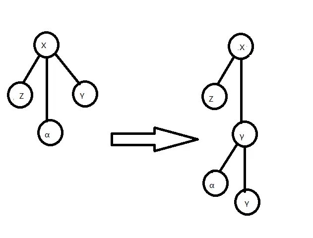
As shown in the figure, this is the process of removing the right child of vertex $x$.

Next comes an alternating sequence of Local Splay and Splice operations. After several Splices, vertex $x$ is rotated to the root of SATT. We analyze one group of Local Splay and Splice operations:

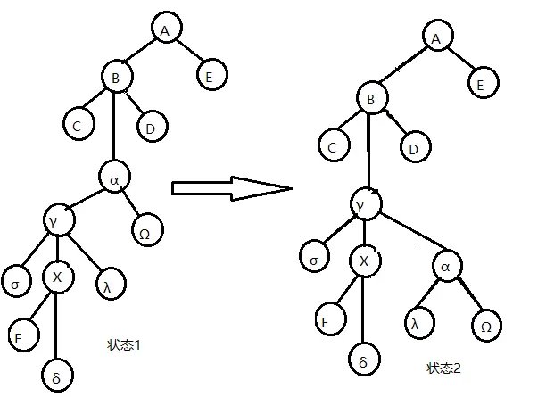
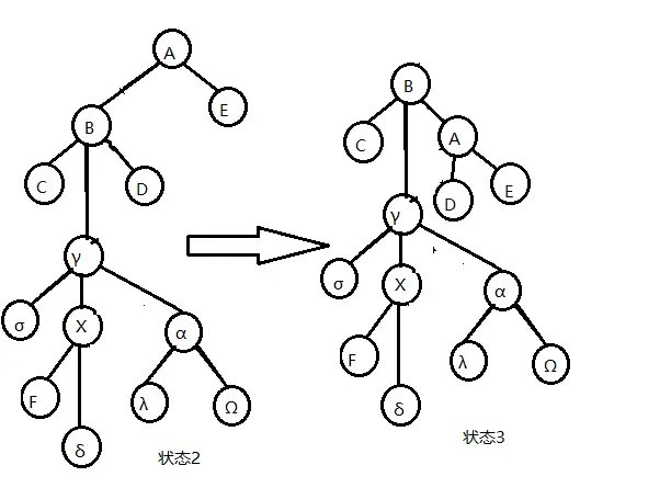
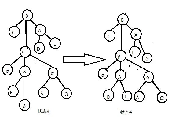
As shown in the figure, this is one Splice operation on vertex $x$, excluding the final step of left-rotating vertex $x$.

For convenience, let $r_x(i)$ be the value of $r$ for vertex $i$ in state $x$.

From the figure, it is easy to see that the amortized complexity of the operation from state 1 to state 2 (the Local Splay operation that rotates the parent of vertex $x$ to the root of its Rake Tree) is

From the figure, it is easy to see that the amortized complexity of the operation from state 2 to state 3 (the Local Splay operation that rotates the grandparent of vertex $x$ to the root of its Compress Tree) is

The key step is to analyze the operation from state 3 to state 4 (Splice):

It is not difficult to see that $r_4(\gamma) \leq r_3(B)$.

Therefore, the amortized complexity of this operation is

Combining the above process, the complexity of one Splice is

Let the value of $r$ for the vertex $X$ of the next Splice (that is, vertex $B$ in state 4) be $r'(X)$. Note that $r_3(\gamma),r_1(\gamma) \ge r_1(X)$, $r_3(B),r_2(\gamma) \leq r'(X)$, and $r_3(B)=r_2(B)$. Therefore,

Besides the complexity above, a Splice may have additional amortized complexity caused by delete(x). Let this part be $a' \leq 3\log n +1$.

Ignoring the $a'$ part for now, the $r'(X)$ of each Splice equals the $r(X)$ of the next one, and the $r(X)$ of the first Splice equals the $r(X)$ when we initially rotate vertex $x$ to the root of its Compress Tree. Thus, excluding delete(x), the complexity of one access(x) is

where $k$ is the number of Splices.

It appears that $a$ contains $3k+1$, making it impossible to analyze the amortized complexity, but we have a way to handle this. Notice that zig-zig/zig-zag rotations can be amortized as follows:

If we can find enough zig-zig and zig-zag operations, we can distribute this $3k+1$ among them and eliminate this $3k+1$..

We find enough zig-zig and zag-zig operations in Global Splay to use, because the number of nodes in Global Splay is certainly greater than $k$, and the number of nodes on the path from vertex $x$ to the root of Global Splay is certainly no less than $k$. In other words, one access(x) must contain at least $\dfrac k2$ zig-zag operations. Including the amortized complexity $a \leq 3\log n +1$ of Global Splay, the amortized complexity of one access(x), excluding delete(x), is

Now include $a'$ and write the total expression for performing $m$ access(x) operations.

What we want is the actual complexity:

Notice that the essence of the delete(x) operation is deleting a Rake Node, but during $m$ operations we add at most $m$ Rake Nodes. By the definition of a Rake Node, there are at most $n$ Rake Nodes initially, so in total we perform at most $m+n$ delete(x) operations. Since $a' \leq 3\log n +1$, we have

Thus, we have proved the complexity of Access. Every other function is either based on Access or has constant single-operation complexity, so we have proved the complexity of SATT.

As an aside, if we omit the Global Splay process as in LCT and instead directly rotate the vertex to be Accessed during each Splice, the time complexity is also correct (in practice, the version without Global Splay is much faster and performs about as well as LCT on Luogu P3690).

Examples

Example 1

To maintain the dynamic diameter, after building SATT, we only need to maintain each vertex's answer in Pushup(x) and finally query the answer at the root (that is, the diameter of the entire tree).

void pushup(int x, int op) {
  if (op == 0) {
    // Compress Node
    len[x] = len[ls(x)] + len[rs(x)];
    diam[x] = maxs[ls(x)][1] + maxs[rs(x)][0];
    diam[x] =
        max(diam[x], max(maxs[ls(x)][1], maxs[rs(x)][0]) + maxs[ms(x)][0]);
    diam[x] = max(diam[x], max(max(diam[ls(x)], diam[rs(x)]), diam[ms(x)]));
    maxs[x][0] =
        max(maxs[ls(x)][0], len[ls(x)] + max(maxs[ms(x)][0], maxs[rs(x)][0]));
    maxs[x][1] =
        max(maxs[rs(x)][1], len[rs(x)] + max(maxs[ms(x)][0], maxs[ls(x)][1]));
  } else {
    // Rake Node
    diam[x] = maxs[ls(x)][0] + maxs[rs(x)][0];
    diam[x] =
        max(diam[x], maxs[ms(x)][0] + max(maxs[ls(x)][0], maxs[rs(x)][0]));
    diam[x] = max(max(diam[x], diam[ms(x)]), max(diam[ls(x)], diam[rs(x)]));
    maxs[x][0] = max(maxs[ms(x)][0], max(maxs[ls(x)][0], maxs[rs(x)][0]));
  }
  return;
}

Here, $diam$ is the answer for the current node (the diameter of the cluster represented by this node). $len$ is the length of the cluster path of the Compress Node's current cluster. $maxs_{0/1}$ is the maximum distance from the Compress Node to an internal node or endpoint of the cluster, excluding the cluster-path child or the parent, respectively (for a Rake Node, only the maximum distance $maxs_0$ from the upper endpoint of the current cluster to an internal node or endpoint is stored). We can simply query the diam of the root node of SATT each time; correctness is evident.

Make some changes to Pushrev(x).

void pushrev(int x) {
  if (!x) return;
  r[x] ^= 1;
  swap(ls(x), rs(x));
  swap(maxs[x][0], maxs[x][1]);
}

Example 2

If we can dynamically maintain the centroid of a tree in $O(\log n)$ time, we can solve this problem.

SATT supports dynamically maintaining a tree's centroid in $O(\log n)$ time. To do this, we need Non-local Search.

For a property on a tree, if a vertex or edge has this property in the entire tree and every subtree containing it also has this property, we call the property Local; otherwise, it is Non-local. Local information can generally be maintained with pushup(x).

For example, the minimum weight is Local: if a vertex or edge has minimum weight in the entire tree, then it also has minimum weight in every subtree containing it. The second-smallest weight is clearly Non-local.

The $diam$ maintained above is also Local information.

Returning to the problem, a centroid is clearly Non-local information and cannot be maintained by a simple pushup(x). We consider searching on SATT:

Our search starts at the root node of SATT, that is, the root cluster. The centroid has a useful property: if one side of an edge contains at least as many vertices as the other side, that side of the edge contains at least one centroid (there may be two centroids).

Let $sum$ denote the number of vertices in a cluster, and let $maxs$ be the maximum $sum$ of the children among all Rake Nodes in a Rake Tree.

void pushup(int x, int op) {
  if (op == 0) {
    // Compress Node
    sum[x] = sum[ls(x)] + sum[rs(x)] + sum[ms(x)] + 1;
  } else {
    // Rake Node
    maxs[x] = max(maxs[ls(x)], max(maxs[rs(x)], sum[ms(x)]));
    sum[x] = sum[ls(x)] + sum[rs(x)] + sum[ms(x)];
  }
}

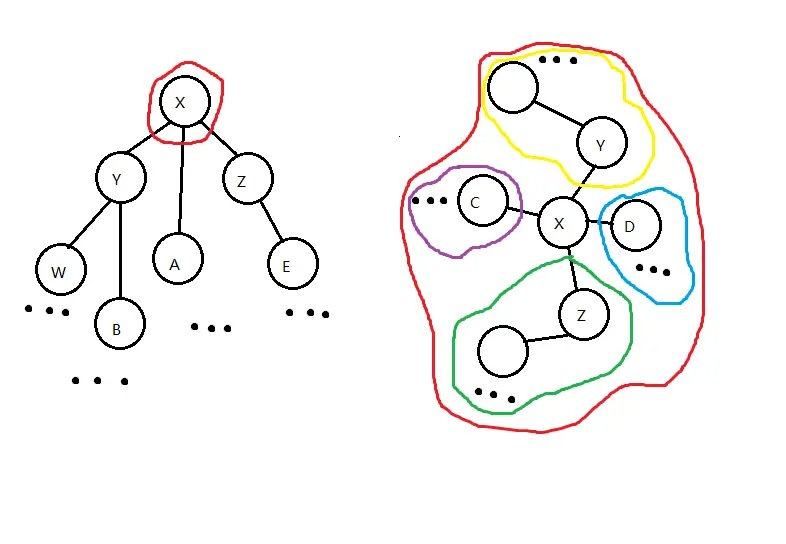
As shown in the figure, this is SATT and the corresponding original tree $T$ during Non-local Search.

We make the following comparisons:

1. Compare the $sum$ of cluster $compress(Y)$ with the $sum$ of the union of cluster $compress(Z)$, cluster $A$, and vertex $X$ (which we temporarily call cluster $\alpha$). If the $sum$ of $compress(Y)$ is greater than or equal to the latter, at least one centroid lies in the subtree of $compress(Y)$, so we recursively search $compress(Y)$. (If they are equal here, vertex $X$ is also a centroid and must be recorded.)

2. Compare the $sum$ of cluster $compress(Z)$ with the $sum$ of the union of cluster $compress(Y)$, cluster $A$, and vertex $X$ (which we temporarily call cluster $\beta$). If the $sum$ of $compress(Z)$ is greater than or equal to the latter, at least one centroid lies in the subtree of $compress(Z)$, so we recursively search $compress(Z)$. (If they are equal here, vertex $X$ is also a centroid and must be recorded.)

3. Compare the $sum$ of the smaller cluster with the largest $sum$ among the Rake tree's middle children of vertex $x$ with the $sum$ of the union of cluster $compress(Y)$, cluster $A$, vertex $X$, and the other smaller clusters (which we temporarily call cluster $Y$). If the $sum$ of that smaller cluster is greater than or equal to the latter, at least one centroid lies in the subtree of that smaller cluster, so we recursively search it. (If they are equal here, vertex $X$ is also a centroid and must be recorded.)

4. If none of the above comparisons leads to a recursive search, vertex $X$ must be a centroid; record it and exit.

The correctness of the first search is clear. How should we search afterward?

Suppose we recurse into $Y$. The information stored by $Y$ is now incomplete, because $compress(Y)$ stores only the information of its own cluster, whereas we need the centroid of the entire tree. The solution is to record the information of the preceding clusters, and when comparing and calculating at vertex $Y$, merge the preceding cluster's information with the information of vertex $Y$ itself. The specific implementation is as follows:

void non_local_search(int x, int lv, int rv, int op) {
  // lv comment rv comment
  if (!x) return;
  psd(x, 0);
  if (op == 0) {
    if (maxs[ms(x)] >=
        sum[ms(x)] - maxs[ms(x)] + sum[rs(x)] + sum[ls(x)] + lv + 1 + rv) {
      if (maxs[ms(x)] ==
          sum[ms(x)] - maxs[ms(x)] + sum[rs(x)] + sum[ls(x)] + lv + 1 + rv) {
        if (ans1)
          ans2 = x;
        else
          ans1 = x;
      }
      non_local_search(
          ms(x),
          sum[ms(x)] - maxs[ms(x)] + sum[rs(x)] + sum[ls(x)] + 1 + lv + rv, 0,
          1);
      return;
    }
    if (ss[rs(x)] + rv >= ss[ms(x)] + ss[ls(x)] + lv + 1) {
      if (ss[rs(x)] + rv == ss[ms(x)] + ss[ls(x)] + lv + 1) {
        if (ans1)
          ans2 = x;
        else
          ans1 = x;
      }
      non_local_search(rs(x), sum[ms(x)] + 1 + sum[ls(x)] + lv, rv, 0);
      return;
    }
    if (sum[ls(x)] + lv >= sum[ms(x)] + sum[rs(x)] + 1 + rv) {
      if (sum[ls(x)] + lv == sum[ms(x)] + sum[rs(x)] + 1 + rv) {
        if (ans1)
          ans2 = x;
        else
          ans1 = x;
      }
      non_local_search(ls(x), lv, rv + sum[ms(x)] + 1 + sum[rs(x)], 0);
      return;
    }
  } else {
    if (maxs[ls(x)] == maxs[x]) {
      non_local_search(ls(x), lv, rv, 1);
      return;
    }
    if (maxs[rs(x)] == maxs[x]) {
      non_local_search(rs(x), lv, rv, 1);
      return;
    }
    non_local_search(ms(x), lv, rv, 0);
    return;
  }
  if (ans1)
    ans2 = x;
  else
    ans1 = x;
}

#include <algorithm>
#include <iostream>
#define ls(x) T[x][0]
#define rs(x) T[x][1]
#define ms(x) T[x][2]
using namespace std;

constexpr int MAXN = 600005;

int T[MAXN][3], tot, r[MAXN], top, st[MAXN], f[MAXN], maxs[MAXN], ss[MAXN];

int nnd() {
  if (top) {
    top--;
    return st[top + 1];
  }
  return ++tot;
}

bool isr(int x) { return rs(f[x]) != x && ls(f[x]) != x; }

bool dir(int x) { return rs(f[x]) == x; }

void psr(int x) {
  if (!x) return;
  r[x] ^= 1;
  swap(ls(x), rs(x));
}

void psd(int x, int ty) {
  if (ty) return;
  if (r[x]) {
    psr(ls(x));
    psr(rs(x));
    r[x] = 0;
  }
}

void psu(int x, int op) {
  psd(x, op); /*comment psd*/
  if (op == 0) {
    ss[x] = ss[ls(x)] + ss[rs(x)] + ss[ms(x)] + 1;
  } else {
    maxs[x] = max(maxs[ls(x)], max(maxs[rs(x)], ss[ms(x)]));
    ss[x] = ss[ls(x)] + ss[rs(x)] + ss[ms(x)];
  }
}

void upd(int x, int ty) {
  if (!isr(x)) upd(f[x], ty);
  psd(x, ty);
}

void stf(int x, int fa, int ty) {
  if (x) f[x] = fa;
  T[fa][ty] = x;
}

void rtt(int x, int ty) {
  int y = f[x], z = f[y], d = dir(x), w = T[x][d ^ 1];
  if (z) T[z][ms(z) == y ? 2 : dir(y)] = x;
  T[x][d ^ 1] = y;
  T[y][d] = w;
  if (w) f[w] = y;
  f[y] = x;
  f[x] = z;
  psu(y, ty);
  psu(x, ty);
}

void spy(int x, int ty, int gl = 0) {
  upd(x, ty);
  for (int y; y = f[x], (!isr(x)) && y != gl; rtt(x, ty)) {
    if (f[y] != gl && (!isr(y))) rtt(dir(x) ^ dir(y) ? x : y, ty);
  }
}

void cle(int x) {
  ls(x) = ms(x) = rs(x) = ss[x] = r[x] = maxs[x] = f[x] = 0;
  st[++top] = x;
}

void del(int x) {
  stf(ms(x), f[x], 1);
  if (ls(x)) {
    int p = ls(x);
    psd(p, 1);
    while (rs(p)) p = rs(p), psd(p, 1);
    spy(p, 1, x);
    stf(rs(x), p, 1);
    stf(p, f[x], 2);
    psu(p, 1);
    psu(f[x], 0);
  } else
    stf(rs(x), f[x], 2);
  cle(x);
}

void spl(int x) {
  spy(x, 1);
  int y = f[x];
  spy(y, 0);
  psd(x, 1);
  if (rs(y)) {
    swap(f[ms(x)], f[rs(y)]);
    swap(ms(x), rs(y));
  } else
    del(x);
  psu(x, 1);
  psu(y, 0);
  rtt(rs(y), 0);
}

void acs(int x) {
  spy(x, 0);
  if (rs(x)) {
    int y = nnd();
    stf(ms(x), y, 0);
    stf(rs(x), y, 2);
    rs(x) = 0;
    stf(y, x, 2);
    psu(y, 1);
    psu(x, 0);
  }
  while (f[x]) spl(f[x]);
}

void mkr(int x) {
  acs(x);
  psr(x);
}

void epo(int x, int y) {
  mkr(x);
  acs(y);
}

void lnk(int x, int y) {
  acs(x);
  mkr(y);
  stf(y, x, 1);
  psu(x, 0);
}

void cu(int x, int y) {
  epo(x, y);
  f[x] = ls(y) = 0;
  psu(y, 0);
}

int ans1, ans2;

void non_local_search(int x, int lv, int rv, int op) {
  if (!x) return;
  psd(x, 0);
  if (op == 0) {
    if (maxs[ms(x)] >=
        ss[ms(x)] - maxs[ms(x)] + ss[rs(x)] + ss[ls(x)] + lv + 1 + rv) {
      if (maxs[ms(x)] ==
          ss[ms(x)] - maxs[ms(x)] + ss[rs(x)] + ss[ls(x)] + lv + 1 + rv) {
        if (ans1)
          ans2 = x;
        else
          ans1 = x;
      }
      non_local_search(
          ms(x), ss[ms(x)] - maxs[ms(x)] + ss[rs(x)] + ss[ls(x)] + 1 + lv + rv,
          0, 1);
      return;
    }
    if (ss[rs(x)] + rv >= ss[ms(x)] + ss[ls(x)] + lv + 1) {
      if (ss[rs(x)] + rv == ss[ms(x)] + ss[ls(x)] + lv + 1) {
        if (ans1)
          ans2 = x;
        else
          ans1 = x;
      }
      non_local_search(rs(x), ss[ms(x)] + 1 + ss[ls(x)] + lv, rv, 0);
      return;
    }
    if (ss[ls(x)] + lv >= ss[ms(x)] + ss[rs(x)] + 1 + rv) {
      if (ss[ls(x)] + lv == ss[ms(x)] + ss[rs(x)] + 1 + rv) {
        if (ans1)
          ans2 = x;
        else
          ans1 = x;
      }
      non_local_search(ls(x), lv, rv + ss[ms(x)] + 1 + ss[rs(x)], 0);
      return;
    }
  } else {
    if (maxs[ls(x)] == maxs[x]) {
      non_local_search(ls(x), lv, rv, 1);
      return;
    }
    if (maxs[rs(x)] == maxs[x]) {
      non_local_search(rs(x), lv, rv, 1);
      return;
    }
    non_local_search(ms(x), lv, rv, 0);
    return;
  }
  if (ans1)
    ans2 = x;
  else
    ans1 = x;
  return;
}

int qu[MAXN], qv[MAXN];

int main() {
  cin.tie(nullptr)->sync_with_stdio(false);
  int TT;
  cin >> TT;
  while (TT--) {
    int n;
    cin >> n;
    tot = n;
    long long ANS = 0;
    for (int i = 1; i <= n; i++) ss[i] = 1;
    for (int i = 1; i < n; i++) {
      cin >> qu[i] >> qv[i];
      lnk(qu[i], qv[i]);
    }
    for (int i = 1; i < n; i++) {
      cu(qu[i], qv[i]);
      ans1 = 0;
      ans2 = 0;
      non_local_search(qu[i], 0, 0, 0);
      ANS += ans1 + ans2;
      if (ans1) acs(ans1);
      if (ans2) acs(ans2);
      ans1 = 0;
      ans2 = 0;
      non_local_search(qv[i], 0, 0, 0);
      ANS += ans1 + ans2;
      if (ans1) acs(ans1);
      if (ans2) acs(ans2);
      lnk(qu[i], qv[i]);
    }
    cout << ANS << '\n';
    for (int i = 1; i <= tot; i++)
      T[i][0] = T[i][1] = T[i][2] = ss[i] = r[i] = maxs[i] = f[i] = 0;
    tot = top = 0;
  }
  return 0;
}

Reference

1. Robert E. Tarjan and Renato F. Werneck. 2005. Self-adjusting top trees. In Proceedings of the sixteenth annual ACM-SIAM symposium on Discrete algorithms (SODA '05). Society for Industrial and Applied Mathematics, USA, 813–822. DOI 10.5555/1070432.1070547

2. negiizhao term