Introduction
Link/Cut Tree is a data structure used to solve dynamic-tree problems.
Link/Cut Tree is also called Link-Cut Tree, abbreviated LCT. It is not itself a dynamic tree; a dynamic tree refers to a class of problems.
Splay Tree is the foundation of LCT, but the Splay Tree used by LCT differs from an ordinary Splay in some details, with several extensions.
Problem introduction
Maintain a tree with the following operations:
- Modify the weights on the path between two vertices.
- Query the sum of weights on the path between two vertices.
- Modify the weights in a vertex subtree.
- Query the sum of weights in a vertex subtree.
This is a standard heavy-light-decomposition problem.
Now add one more operation:
- Cut and link edges while preserving the tree property.
The answers must be produced online.
This becomes a dynamic-tree problem, which can be solved with LCT.
Dynamic-tree problem
Maintain a forest while supporting deletion and insertion of edges, with the guarantee that the result remains a forest after every operation. We need to maintain some information about this forest.
Common operations include checking connectivity between two vertices, querying path-weight sums, linking two vertices, cutting an edge, and modifying information.
Heavy-light decomposition from the LCT viewpoint
- Decompose the whole tree according to subtree sizes and relabel the vertices.
- After relabeling, we obtain contiguous intervals on the tree whose units are chains, so segment trees can perform interval operations.
Turning to dynamic-tree problems
The decomposition just described uses subtree size as its criterion. Can we redefine the decomposition so that it is better suited to dynamic-tree problems?
Let us consider what kind of chains a dynamic-tree problem needs.
Because the forest is maintained dynamically, we naturally want these to be chains of our own choice, so that we can use them in the solution.
Preferred-path decomposition
For the edges from a vertex to all its children, we choose one edge for the decomposition. We call the chosen edge a preferred edge and the others virtual edges; the child connected by a preferred edge is a preferred child. A chain consisting of preferred edges is likewise a preferred path. Remember the most important reason for choosing this decomposition: the preferred paths are chosen by us and can change flexibly. It is precisely this flexibility that lets us use Splay Trees to maintain them.
LCT
We can simply view LCT as using several Splay Trees to maintain a dynamic tree decomposition, enabling interval operations on dynamic trees. For each preferred path, we build a Splay Tree to maintain the information for the entire path interval.
Auxiliary tree
Let us first examine some properties of auxiliary trees, and then use a diagram to understand their concrete structure.
In this article, you can think of several Splay Trees as forming an auxiliary tree. Each auxiliary tree maintains one tree, and several auxiliary trees form an LCT that maintains the entire forest.
- An auxiliary tree consists of several Splay Trees, each maintaining a path in the original tree. The vertex sequence obtained by an in-order traversal of a Splay corresponds, from front to back, to a path in the original tree from top to bottom.
- Each vertex of the original tree corresponds one-to-one with a Splay node in the auxiliary tree.
- The Splay Trees in an auxiliary tree are not independent. The parent of each Splay root would normally be null, but in an LCT it points to the parent of this path in the original tree (that is, the parent of the topmost vertex on the path). This parent link differs from an ordinary Splay parent link: the child recognizes the parent, but the parent does not recognize the child. It represents a virtual edge of the original tree. Therefore, each connected component has exactly one vertex whose parent is null.
- Because of these properties, maintaining an operation never requires maintaining the original tree explicitly. The auxiliary trees uniquely determine an original tree in every state, so we only need to maintain the auxiliary trees.
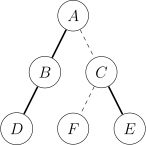
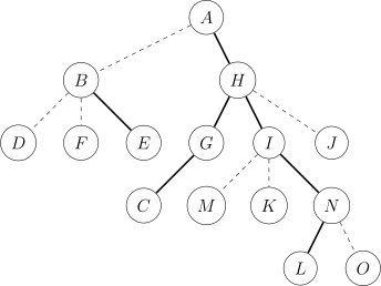
Here is an original tree, as shown in the figure. (Bold edges are preferred edges, and dashed edges are virtual edges.)
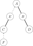
By the definition above, the auxiliary tree has the structure shown in the figure.
Relationship between the original and auxiliary trees
- A preferred path in the original tree: its vertices all lie in one Splay Tree in the auxiliary tree.
- A virtual path in the original tree: in the auxiliary tree, the Splay containing the child points to the parent through Father, but neither child pointer of the parent points to the child.
- Note that the root of the original tree is not the root of the auxiliary tree.
- The Father pointer in the original tree is not the same as the Father pointer in the auxiliary tree.
- An auxiliary tree can be rerooted arbitrarily while preserving the auxiliary-tree and Splay properties.
- Preferred/virtual path transformations can be completed easily in the auxiliary tree; this is what enables dynamic maintenance of the tree decomposition.
Variables used below
ch[N][2]left and right childrenf[N]parent pointersum[N]path-weight sumval[N]vertex weighttag[N]reversal taglaz[N]weight tagsiz[N]subtree size in the auxiliary tree- Other_Vars
Function declarations
General data-structure functions (literal meanings)
PushUp(x)PushDown(x)
Splay-tree functions
The following functions are used in Splay Trees; see Splay tree for details.
Get(x)obtains which child of its parent is.Splay(x)works together with Rotate to rotate to the root of the current Splay.Rotate(x)rotates upward by one level.
New operations
Access(x)puts every vertex from the root to on one preferred path, so the root-to- path becomes a preferred path in one Splay Tree. Only this operation is mandatory; implement the others as required by the problem.IsRoot(x)determines whether is the root of its tree.Update(x)after anAccessoperation recursively callsPushDownfrom top to bottom to update the information.MakeRoot(x)makes vertex the root of its tree.Link(x, y)adds an edge between .Cut(x, y)removes the edge between .Find(x)finds the index of the root of the tree containing .Fix(x, v)changes the vertex weight of to .Split(x, y)extracts the path between for interval operations.
Macro definitions
#define ls ch[p][0]#define rs ch[p][1]
Function explanations
PushUp()
void PushUp(int p) {
  // maintain other variables
  siz[p] = siz[ls] + siz[rs] + 1;
}
PushDown()
void PushDown(int p) {
  if (tag[p] != std_tag) {
    // pushdown the tag
    tag[p] = std_tag;
  }
}
Splay() && Rotate()
The implementations of Splay() and Rotate() here differ somewhat from those in a Splay tree.
#define Get(x) (ch[f[x]][1] == x)

void Rotate(int x) {
  int y = f[x], z = f[y], k = Get(x);
  if (!isRoot(y)) ch[z][ch[z][1] == y] = x;
  // This line must come first. An ordinary Splay does not need it because of isRoot (explained below).
  ch[y][k] = ch[x][!k], f[ch[x][!k]] = y;
  ch[x][!k] = y, f[y] = x, f[x] = z;
  PushUp(y), PushUp(x);
}

void Splay(int x) {
  Update(
      x);  // As will be clear shortly, PushDown every vertex on the path traversed by the rotations before Splay.
  for (int fa; fa = f[x], !isRoot(x); Rotate(x)) {
    if (!isRoot(fa)) Rotate(Get(fa) == Get(x) ? fa : x);
  }
}
For the functions above, see Splay tree.
The following functions are specific to LCT.
isRoot()
// As mentioned earlier, in an LCT, if a child is not a preferred child, its parent cannot find it.
// Therefore, when a vertex is neither the left nor the right child of its parent, it is the root of the current Splay.
#define isRoot(x) (ch[f[x]][0] != x && ch[f[x]][1] != x)
Access()
// Access is the core operation of an LCT.
// Suppose we want to process a path and that path happens to be our current Splay;
// we can use its information directly. Let us first look at the code and then the process in the figures.
int Access(int x) {
  int p;
  for (p = 0; x; p = x, x = f[x]) {
    Splay(x), ch[x][1] = p, PushUp(x);
  }
  return p;
}
-
Consider a tree in which solid lines are preferred edges and dashed lines are virtual edges.
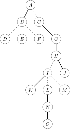
initial tree -
Its auxiliary tree may look like this (different drawings may produce different LCT structures).
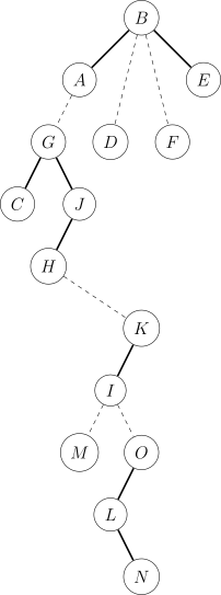
initial auxtree -
We now perform
Access(N), turning every edge on the path from to into a preferred edge and pulling it into one Splay Tree.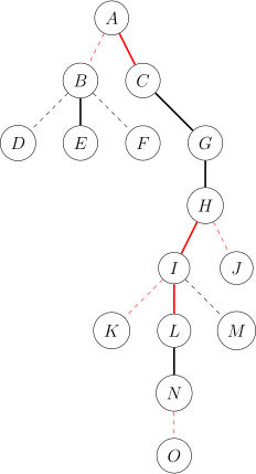
access tree -
The operation is implemented by updating the Splay Trees step by step from bottom to top.
-
First, rotate to the root of its current Splay.
-
To preserve the properties of the AuxTree, the former preferred edge from to must be changed into a virtual edge.
-
Because the child recognizes the parent but not vice versa, we can simply change the child of to
NULL. -
Thus the original AuxTree changes from the figure below to the next figure.
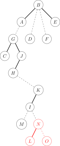
step 1 auxtree -
Next, rotate 's Father to the root of the Splay Tree rooted at .
-
Remove the former preferred edge —. Then point the right child of to , obtaining the Splay shown as —.
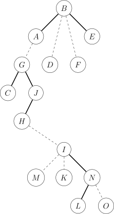
step 2 auxtree -
Next, following the same steps, because the Father of points to , rotate to the root of its Splay Tree and set the rs of to .
-
The tree then looks like this.
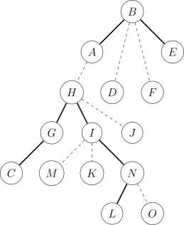
step 3 auxtree -
Similarly, perform
Splay(A)and point the right child of to . -
We obtain the AuxTree shown here, and the entire path from to is now in the same Splay Tree.
step final auxtree
// Review the code.
int Access(int x) {
  int p;
  for (p = 0; x; p = x, x = f[x]) {
    Splay(x), ch[x][1] = p, PushUp(x);
  }
  return p;
}
Access() is actually simple; it consists of the following four steps:
- Rotate the current node to the root.
- Replace its child with the previously processed node.
- Update the information of the current vertex.
- Replace the current vertex with its parent and continue.
The Access presented here also has a return value. It is the index of the virtual-edge parent vertex in the last preferred/virtual path transformation. It has two meanings:
- For two consecutive Access operations, the return value of the second operation is the LCA of the two vertices.
- It represents the root of the Splay Tree containing the path from to the root. This vertex has already been rotated to the root, and its parent is necessarily null.
Update()
// PushDown one level at a time from top to bottom.
void Update(int p) {
  if (!isRoot(p)) Update(f[p]);
  pushDown(p);
}
makeRoot()
Make_Root()is just as important asAccess(). When maintaining path information, we may encounter a path whose depths do not increase strictly; by the properties of an AuxTree, such a path cannot appear in one Splay Tree.- This is when we need
Make_Root(). Make_Root()makes the specified vertex the root of the original tree; let us consider how to implement it.- Suppose the return value of
Access(x)is . The path from to the current root then forms exactly one Splay, whose root is . - Represent the tree as a directed graph, orienting every edge from child to parent. It is easy to see that rerooting reverses every edge on the path from to the root (think this through carefully).
- Therefore, we only need to reverse the path from to the current root.
- Since is the root of the Splay representing the path from to the current root, we can reverse the interval of the Splay rooted at .
void makeRoot(int p) {
  p = Access(p);
  swap(ch[p][0], ch[p][1]);
  tag[p] ^= 1;
}
Link()
Linking two vertices is simple: first call Make_Root(x), then make the parent of point to . Clearly, this operation cannot be performed within the same tree, so remember to check that first.
void Link(int x, int p) {
  makeRoot(x);
  splay(x);
  f[x] = p;
}
Split()
- The meaning of
Splitis simple: extract one Splay Tree that maintains the path from to . - First call
MakeRoot(x), thenAccess(y). If is to be the root, callSplay(y)as well. - These three operations in Split directly bring the required path into the subtree of , where other operations can be performed.
Cut()
Cuthas two cases: the operation may or may not be guaranteed to be valid.- If validity is guaranteed, call
Split(x, y)directly. Then is the root and must be its child, so disconnect them in both directions, as follows:
void Cut(int x, int p) { makeRoot(x), Access(p), Splay(p), ls = f[x] = 0; }
If validity is not guaranteed, we need to check whether the edge exists. One option is to store the edges in a map, but the following method uses the structural properties:
To delete an edge, the following three conditions must hold:
- are connected.
- There is no other path on the path between .
- has no right child.
In short, the three statements above simply mean that there is an edge between .
The implementation is left as an exercise. Connectivity is checked using the Find described below; with a little structural analysis, the other two conditions are straightforward to test.
Find()
Find()searches for the root of the original tree containing ; do not confuse it with the root of the auxiliary tree. AfterAccess(p), callSplay(p). The root is then the vertex of minimum depth in the tree; keep moving to the left child and callPushDownalong the way.- Continue until there is no ls; it is that simple.
- Note that after every query, the vertex corresponding to the answer must be brought up with
Splayto preserve the complexity bound.
int Find(int p) {
  Access(p);
  Splay(p);
  pushDown(p);
  while (ls) p = ls, pushDown(p);
  Splay(p);
  return p;
}
Notes
- Before each operation, consider whether
PushUporPushDownis needed. Because LCT is especially flexible, omitting even onePushdownorPushupmay apply an update to the wrong vertex. - LCT's
Rotatediffers from Splay's;if (z)must come first. - LCT's
Splayoperation always rotates to the root; there is no operation to rotate to a particular child because it is unnecessary.
Time complexity
Most LCT operations are based on Access, while the remaining operations take constant time. Thus, we only need to analyze the time complexity of Access.
The time complexity of Access mainly comes from repeated Splay operations and from traversing virtual edges on the path. We analyze these two parts separately.
-
Splay
-
Define , where is the total number of virtual and preferred edges in the tree rooted at .
-
Define the potential function , where is the set of all vertices.
From the analysis of Splay time complexity, the amortized time complexity of a Splay operation is .
-
-
Traversing virtual edges
Following heavy-light decomposition, define two kinds of virtual edges:
-
Heavy virtual edge: a virtual edge from vertex to its parent, with .
-
Light virtual edge: a virtual edge from vertex to its parent, with .
Virtual edges can be handled with potential analysis. Define the potential as the number of heavy virtual edges, and define the amortized cost as , where is the actual operation cost and is the change in potential.
-
After traversing a heavy virtual edge, it becomes a preferred edge. This reduces the potential by , since it improves the tree structure by strengthening an important connection. Its actual cost is , which offsets the increase in potential, so it does not increase the amortized cost; all amortized cost is concentrated in processing light virtual edges.
-
Each
Accessoperation traverses at most light virtual edges, so it incurs at most actual cost and creates heavy virtual edges; equivalently, the potential increases by .
Therefore, the amortized complexity of traversing virtual edges is the sum of the actual cost and the potential change, namely .
-
In summary, the time complexity of Access in an LCT is the sum of the complexities of Splay operations and virtual-edge traversals, so its amortized complexity is . For an LCT with n vertices, m Access operations take time. Consequently, operations based on Access, such as Cut, Link, and Findroot, also have amortized complexity .
Exercises
Maintaining path information
Using Split(x,y), LCT can extract the path from to in the tree into a Splay rooted at . Updates and queries of path information then become operations on a balanced tree, which gives LCT an advantage for maintaining path information. In addition, binary search on a path implemented with LCT is lower by a factor of in complexity than binary search with heavy-light decomposition.
Example problem: "National Training Team" Tree II
Given a tree with vertices, each initially having weight . There are operations, each of which is one of the following four types:
-
- u1 v1 u2 v2: Delete the edge between in the tree, then connect , with the guarantee that the operation is valid and the result is still a tree. -
+ u v c: Increase all vertex weights on the path between by . -
* u v c: Multiply all vertex weights on the path between by . -
/ u v: Output the sum of vertex weights on the path between , modulo .The
-operation can be implemented directly asCut(u1,v1),Link(u2,v2).
When modifying the path between in the tree, first call Split(u,v).
This problem requires subtree addition, subtree multiplication, and subtree-sum queries in the auxiliary tree. Therefore, besides the subtree-reversal tag normally maintained by an LCT, we must also maintain subtree-addition and subtree-multiplication tags. The tags are handled in the same way as in a Splay Tree.
When applying and pushing down an addition tag, the change in the subtree weight sum depends on the number of vertices in the subtree, so we must also maintain the subtree size siz.
When pushing down tags, note the order: push down the multiplication tag before the addition tag. Subtree reversal does not conflict with the subtree addition and multiplication tags.
Reference implementation
#include <algorithm>
#include <cstdio>
#include <cstring>
using namespace std;
constexpr long long MAXN = 100010;
constexpr long long mod = 51061;
long long n, q, u, v, c;
char op;

struct Splay {
  long long ch[MAXN][2], fa[MAXN], siz[MAXN], val[MAXN], sum[MAXN], rev[MAXN],
      add[MAXN], mul[MAXN];

  void clear(long long x) {
    ch[x][0] = ch[x][1] = fa[x] = siz[x] = val[x] = sum[x] = rev[x] = add[x] =
        0;
    mul[x] = 1;
  }

  long long getch(long long x) { return (ch[fa[x]][1] == x); }

  long long isroot(long long x) {
    clear(0);
    return ch[fa[x]][0] != x && ch[fa[x]][1] != x;
  }

  void maintain(long long x) {
    clear(0);
    siz[x] = (siz[ch[x][0]] + 1 + siz[ch[x][1]]) % mod;
    sum[x] = (sum[ch[x][0]] + val[x] + sum[ch[x][1]]) % mod;
  }

  void pushdown(long long x) {
    clear(0);
    if (mul[x] != 1) {
      if (ch[x][0])
        mul[ch[x][0]] = (mul[x] * mul[ch[x][0]]) % mod,
        val[ch[x][0]] = (val[ch[x][0]] * mul[x]) % mod,
        sum[ch[x][0]] = (sum[ch[x][0]] * mul[x]) % mod,
        add[ch[x][0]] = (add[ch[x][0]] * mul[x]) % mod;
      if (ch[x][1])
        mul[ch[x][1]] = (mul[x] * mul[ch[x][1]]) % mod,
        val[ch[x][1]] = (val[ch[x][1]] * mul[x]) % mod,
        sum[ch[x][1]] = (sum[ch[x][1]] * mul[x]) % mod,
        add[ch[x][1]] = (add[ch[x][1]] * mul[x]) % mod;
      mul[x] = 1;
    }
    if (add[x]) {
      if (ch[x][0])
        add[ch[x][0]] = (add[ch[x][0]] + add[x]) % mod,
        val[ch[x][0]] = (val[ch[x][0]] + add[x]) % mod,
        sum[ch[x][0]] = (sum[ch[x][0]] + add[x] * siz[ch[x][0]] % mod) % mod;
      if (ch[x][1])
        add[ch[x][1]] = (add[ch[x][1]] + add[x]) % mod,
        val[ch[x][1]] = (val[ch[x][1]] + add[x]) % mod,
        sum[ch[x][1]] = (sum[ch[x][1]] + add[x] * siz[ch[x][1]] % mod) % mod;
      add[x] = 0;
    }
    if (rev[x]) {
      if (ch[x][0]) rev[ch[x][0]] ^= 1, swap(ch[ch[x][0]][0], ch[ch[x][0]][1]);
      if (ch[x][1]) rev[ch[x][1]] ^= 1, swap(ch[ch[x][1]][0], ch[ch[x][1]][1]);
      rev[x] = 0;
    }
  }

  void update(long long x) {
    if (!isroot(x)) update(fa[x]);
    pushdown(x);
  }

  void print(long long x) {
    if (!x) return;
    pushdown(x);
    print(ch[x][0]);
    printf("%lld ", x);
    print(ch[x][1]);
  }

  void rotate(long long x) {
    long long y = fa[x], z = fa[y], chx = getch(x), chy = getch(y);
    fa[x] = z;
    if (!isroot(y)) ch[z][chy] = x;
    ch[y][chx] = ch[x][chx ^ 1];
    fa[ch[x][chx ^ 1]] = y;
    ch[x][chx ^ 1] = y;
    fa[y] = x;
    maintain(y);
    maintain(x);
    maintain(z);
  }

  void splay(long long x) {
    update(x);
    for (long long f = fa[x]; f = fa[x], !isroot(x); rotate(x))
      if (!isroot(f)) rotate(getch(x) == getch(f) ? f : x);
  }

  void access(long long x) {
    for (long long f = 0; x; f = x, x = fa[x])
      splay(x), ch[x][1] = f, maintain(x);
  }

  void makeroot(long long x) {
    access(x);
    splay(x);
    swap(ch[x][0], ch[x][1]);
    rev[x] ^= 1;
  }

  long long find(long long x) {
    access(x);
    splay(x);
    while (ch[x][0]) x = ch[x][0];
    splay(x);
    return x;
  }
} st;

main() {
  scanf("%lld%lld", &n, &q);
  for (long long i = 1; i <= n; i++) st.val[i] = 1, st.maintain(i);
  for (long long i = 1; i < n; i++) {
    scanf("%lld%lld", &u, &v);
    if (st.find(u) != st.find(v)) st.makeroot(u), st.fa[u] = v;
  }
  while (q--) {
    scanf(" %c%lld%lld", &op, &u, &v);
    if (op == '+') {
      scanf("%lld", &c);
      st.makeroot(u), st.access(v), st.splay(v);
      st.val[v] = (st.val[v] + c) % mod;
      st.sum[v] = (st.sum[v] + st.siz[v] * c % mod) % mod;
      st.add[v] = (st.add[v] + c) % mod;
    }
    if (op == '-') {
      st.makeroot(u);
      st.access(v);
      st.splay(v);
      if (st.ch[v][0] == u && !st.ch[u][1]) st.ch[v][0] = st.fa[u] = 0;
      scanf("%lld%lld", &u, &v);
      if (st.find(u) != st.find(v)) st.makeroot(u), st.fa[u] = v;
    }
    if (op == '*') {
      scanf("%lld", &c);
      st.makeroot(u), st.access(v), st.splay(v);
      st.val[v] = st.val[v] * c % mod;
      st.sum[v] = st.sum[v] * c % mod;
      st.mul[v] = st.mul[v] * c % mod;
    }
    if (op == '/')
      st.makeroot(u), st.access(v), st.splay(v), printf("%lld\n", st.sum[v]);
  }
  return 0;
}
Exercises
- luogu P3690 Link-Cut Tree (dynamic tree) template
- "SDOI2011" Coloring
- "SHOI2014" Ternary Neural Tree
Maintaining connectivity
Checking connectivity
Using the LCT function Find(), we can determine whether two vertices in the dynamic forest are connected. If Find(x)==Find(y), then belong to the same tree and are connected.
Example problem: "SDOI2008" Cave Survey
Initially there are isolated vertices and operations. Each operation is one of the following:
Connect u v: Add an edge between .Destroy u v: Delete the edge between ; such an edge is guaranteed to have existed previously.Query u v: Ask whether are connected.
The graph is guaranteed to be a forest at every moment.
Reference implementation
#include <algorithm>
#include <cstdio>
#include <cstring>
using namespace std;
constexpr int MAXN = 10010;

struct Splay {
  int ch[MAXN][2], fa[MAXN], tag[MAXN];

  void clear(int x) { ch[x][0] = ch[x][1] = fa[x] = tag[x] = 0; }

  int getch(int x) { return ch[fa[x]][1] == x; }

  int isroot(int x) { return ch[fa[x]][0] != x && ch[fa[x]][1] != x; }

  void pushdown(int x) {
    if (tag[x]) {
      if (ch[x][0]) swap(ch[ch[x][0]][0], ch[ch[x][0]][1]), tag[ch[x][0]] ^= 1;
      if (ch[x][1]) swap(ch[ch[x][1]][0], ch[ch[x][1]][1]), tag[ch[x][1]] ^= 1;
      tag[x] = 0;
    }
  }

  void update(int x) {
    if (!isroot(x)) update(fa[x]);
    pushdown(x);
  }

  void rotate(int x) {
    int y = fa[x], z = fa[y], chx = getch(x), chy = getch(y);
    fa[x] = z;
    if (!isroot(y)) ch[z][chy] = x;
    ch[y][chx] = ch[x][chx ^ 1];
    fa[ch[x][chx ^ 1]] = y;
    ch[x][chx ^ 1] = y;
    fa[y] = x;
  }

  void splay(int x) {
    update(x);
    for (int f = fa[x]; f = fa[x], !isroot(x); rotate(x))
      if (!isroot(f)) rotate(getch(x) == getch(f) ? f : x);
  }

  void access(int x) {
    for (int f = 0; x; f = x, x = fa[x]) splay(x), ch[x][1] = f;
  }

  void makeroot(int x) {
    access(x);
    splay(x);
    swap(ch[x][0], ch[x][1]);
    tag[x] ^= 1;
  }

  int find(int x) {
    access(x);
    splay(x);
    while (ch[x][0]) x = ch[x][0];
    splay(x);
    return x;
  }
} st;

int n, q, x, y;
char op[MAXN];

int main() {
  scanf("%d%d", &n, &q);
  while (q--) {
    scanf("%s%d%d", op, &x, &y);
    if (op[0] == 'Q') {
      if (st.find(x) == st.find(y))
        printf("Yes\n");
      else
        printf("No\n");
    }
    if (op[0] == 'C')
      if (st.find(x) != st.find(y)) st.makeroot(x), st.fa[x] = y;
    if (op[0] == 'D') {
      st.makeroot(x);
      st.access(y);
      st.splay(y);
      if (st.ch[y][0] == x && !st.ch[x][1]) st.ch[y][0] = st.fa[x] = 0;
    }
  }
  return 0;
}
Maintaining edge-biconnected components
If edge-biconnected components are to be contracted into vertices, then whenever an edge is added, if its two endpoints are already connected in the tree, every vertex on the path between them is contracted into one vertex.
Example problem: "AHOI2005" Route Planning
Given vertices, initially with undirected edges, and operations, each of which is one of the following:
0 u v: Delete the edge between ; such an edge is guaranteed to exist at that time.1 u v: Query the number of edges that every possible path between at that time must pass through.
The graph is guaranteed to remain connected at all times.
The number of edges that every possible path between must pass through equals the number of vertices on the path between the vertices containing and after all edge-biconnected components have been contracted, minus .
Because edge deletion is difficult to perform in this problem, we process the operations offline in reverse, turning deletions into additions.
When adding an edge, if its endpoints were originally disconnected, link them in the LCT. Otherwise, extract the path between them in the LCT before the edge was added. Traversing this subtree of the auxiliary tree is equivalent to traversing the path; merge these vertices and use a disjoint-set union structure to maintain the merged information.
Replace the original tree path with the representative element of the merged disjoint-set component. Note that every subsequent operation must use the disjoint-set representative of each operation vertex.
Reference implementation
#include <algorithm>
#include <cstdio>
#include <cstring>
#include <map>
using namespace std;
constexpr int MAXN = 200010;
int f[MAXN];

int findp(int x) { return f[x] ? f[x] = findp(f[x]) : x; }

void merge(int x, int y) {
  x = findp(x);
  y = findp(y);
  if (x != y) f[x] = y;
}

struct Splay {
  int ch[MAXN][2], fa[MAXN], tag[MAXN], siz[MAXN];

  void clear(int x) { ch[x][0] = ch[x][1] = fa[x] = tag[x] = siz[x] = 0; }

  int getch(int x) { return ch[findp(fa[x])][1] == x; }

  int isroot(int x) {
    return ch[findp(fa[x])][0] != x && ch[findp(fa[x])][1] != x;
  }

  void maintain(int x) {
    clear(0);
    if (x) siz[x] = siz[ch[x][0]] + 1 + siz[ch[x][1]];
  }

  void pushdown(int x) {
    if (tag[x]) {
      if (ch[x][0]) tag[ch[x][0]] ^= 1, swap(ch[ch[x][0]][0], ch[ch[x][0]][1]);
      if (ch[x][1]) tag[ch[x][1]] ^= 1, swap(ch[ch[x][1]][0], ch[ch[x][1]][1]);
      tag[x] = 0;
    }
  }

  void print(int x) {
    if (!x) return;
    pushdown(x);
    print(ch[x][0]);
    printf("%d ", x);
    print(ch[x][1]);
  }

  void update(int x) {
    if (!isroot(x)) update(findp(fa[x]));
    pushdown(x);
  }

  void rotate(int x) {
    x = findp(x);
    int y = findp(fa[x]), z = findp(fa[y]), chx = getch(x), chy = getch(y);
    fa[x] = z;
    if (!isroot(y)) ch[z][chy] = x;
    ch[y][chx] = ch[x][chx ^ 1];
    fa[ch[x][chx ^ 1]] = y;
    ch[x][chx ^ 1] = y;
    fa[y] = x;
    maintain(y);
    maintain(x);
    if (z) maintain(z);
  }

  void splay(int x) {
    x = findp(x);
    update(x);
    for (int f = findp(fa[x]); f = findp(fa[x]), !isroot(x); rotate(x))
      if (!isroot(f)) rotate(getch(x) == getch(f) ? f : x);
  }

  void access(int x) {
    for (int f = 0; x; f = x, x = findp(fa[x]))
      splay(x), ch[x][1] = f, maintain(x);
  }

  void makeroot(int x) {
    x = findp(x);
    access(x);
    splay(x);
    tag[x] ^= 1;
    swap(ch[x][0], ch[x][1]);
  }

  int find(int x) {
    x = findp(x);
    access(x);
    splay(x);
    while (ch[x][0]) x = ch[x][0];
    splay(x);
    return x;
  }

  void dfs(int x) {
    pushdown(x);
    if (ch[x][0]) dfs(ch[x][0]), merge(ch[x][0], x);
    if (ch[x][1]) dfs(ch[x][1]), merge(ch[x][1], x);
  }
} st;

int n, m, q, x, y, cur, ans[MAXN];

struct oper {
  int op, a, b;
} s[MAXN];

map<pair<int, int>, int> mp;

int main() {
  scanf("%d%d", &n, &m);
  for (int i = 1; i <= n; i++) st.maintain(i);
  for (int i = 1; i <= m; i++)
    scanf("%d%d", &x, &y), mp[{x, y}] = mp[{y, x}] = 1;
  while (scanf("%d", &s[++q].op)) {
    if (s[q].op == -1) {
      q--;
      break;
    }
    scanf("%d%d", &s[q].a, &s[q].b);
    if (!s[q].op) mp[{s[q].a, s[q].b}] = mp[{s[q].b, s[q].a}] = 0;
  }
  reverse(s + 1, s + q + 1);
  for (map<pair<int, int>, int>::iterator it = mp.begin(); it != mp.end(); it++)
    if (it->second) {
      mp[{it->first.second, it->first.first}] = 0;
      x = findp(it->first.first);
      y = findp(it->first.second);
      if (st.find(x) != st.find(y))
        st.makeroot(x), st.fa[x] = y;
      else {
        if (x == y) continue;
        st.makeroot(x);
        st.access(y);
        st.splay(y);
        st.dfs(y);
        int t = findp(y);
        st.fa[t] = findp(st.fa[y]);
        st.ch[t][0] = st.ch[t][1] = 0;
        st.maintain(t);
      }
    }
  for (int i = 1; i <= q; i++) {
    if (s[i].op == 0) {
      x = findp(s[i].a);
      y = findp(s[i].b);
      st.makeroot(x);
      st.access(y);
      st.splay(y);
      st.dfs(y);
      int t = findp(y);
      st.fa[t] = st.fa[y];
      st.ch[t][0] = st.ch[t][1] = 0;
      st.maintain(t);
    }
    if (s[i].op == 1) {
      x = findp(s[i].a);
      y = findp(s[i].b);
      st.makeroot(x);
      st.access(y);
      st.splay(y);
      ans[++cur] = st.siz[y] - 1;
    }
  }
  for (int i = cur; i >= 1; i--) printf("%d\n", ans[i]);
  return 0;
}
Exercises
Maintaining edge weights
LCT cannot handle edge weights directly. We therefore create a corresponding vertex for each edge, making it convenient to query edge information on a path. This technique can be used to maintain a spanning tree dynamically.
Example problem: luogu P4234 Minimum Difference Spanning Tree
Given a weighted undirected graph with vertices and edges, find a spanning tree minimizing the difference between its maximum and minimum edge weights, and output this difference.
The input is guaranteed to contain at least one spanning tree.
Sort the edges in increasing order of weight and enumerate the selected rightmost edge. To obtain the optimum, we need to maximize the weight of the minimum-weight edge.
Add edges in order. If the two endpoints to be connected are already connected, remove the minimum-weight edge on their path. If the whole graph has become a tree, update the answer with the current edge weight minus the minimum edge weight. The minimum edge weight can be maintained with a two-pointer method.
An LCT has no fixed parent-child relationships, so edge weights cannot be stored as vertex weights.
To record edge information on a tree path, use edge splitting. Create a corresponding vertex for each edge and connect it to the edge's two endpoints; each original link or cut operation then becomes two operations.
Reference implementation
#include <algorithm>
#include <cstdio>
#include <cstring>
#include <set>
using namespace std;
constexpr int MAXN = 5000010;

struct Splay {
  int ch[MAXN][2], fa[MAXN], tag[MAXN], val[MAXN], minn[MAXN];

  void clear(int x) {
    ch[x][0] = ch[x][1] = fa[x] = tag[x] = val[x] = minn[x] = 0;
  }

  int getch(int x) { return ch[fa[x]][1] == x; }

  int isroot(int x) { return ch[fa[x]][0] != x && ch[fa[x]][1] != x; }

  void maintain(int x) {
    if (!x) return;
    minn[x] = x;
    if (ch[x][0]) {
      if (val[minn[ch[x][0]]] < val[minn[x]]) minn[x] = minn[ch[x][0]];
    }
    if (ch[x][1]) {
      if (val[minn[ch[x][1]]] < val[minn[x]]) minn[x] = minn[ch[x][1]];
    }
  }

  void pushdown(int x) {
    if (tag[x]) {
      if (ch[x][0]) tag[ch[x][0]] ^= 1, swap(ch[ch[x][0]][0], ch[ch[x][0]][1]);
      if (ch[x][1]) tag[ch[x][1]] ^= 1, swap(ch[ch[x][1]][0], ch[ch[x][1]][1]);
      tag[x] = 0;
    }
  }

  void update(int x) {
    if (!isroot(x)) update(fa[x]);
    pushdown(x);
  }

  void print(int x) {
    if (!x) return;
    pushdown(x);
    print(ch[x][0]);
    printf("%d ", x);
    print(ch[x][1]);
  }

  void rotate(int x) {
    int y = fa[x], z = fa[y], chx = getch(x), chy = getch(y);
    fa[x] = z;
    if (!isroot(y)) ch[z][chy] = x;
    ch[y][chx] = ch[x][chx ^ 1];
    fa[ch[x][chx ^ 1]] = y;
    ch[x][chx ^ 1] = y;
    fa[y] = x;
    maintain(y);
    maintain(x);
    if (z) maintain(z);
  }

  void splay(int x) {
    update(x);
    for (int f = fa[x]; f = fa[x], !isroot(x); rotate(x))
      if (!isroot(f)) rotate(getch(x) == getch(f) ? f : x);
  }

  void access(int x) {
    for (int f = 0; x; f = x, x = fa[x]) splay(x), ch[x][1] = f, maintain(x);
  }

  void makeroot(int x) {
    access(x);
    splay(x);
    tag[x] ^= 1;
    swap(ch[x][0], ch[x][1]);
  }

  int find(int x) {
    access(x);
    splay(x);
    while (ch[x][0]) x = ch[x][0];
    splay(x);
    return x;
  }

  void link(int x, int y) {
    makeroot(x);
    fa[x] = y;
  }

  void cut(int x, int y) {
    makeroot(x);
    access(y);
    splay(y);
    ch[y][0] = fa[x] = 0;
    maintain(y);
  }
} st;

constexpr int inf = 2e9 + 1;
int n, m, ans, nww, x, y;

struct Edge {
  int u, v, w;

  bool operator<(Edge x) const { return w < x.w; };
} s[MAXN];

multiset<int> mp;

int main() {
  scanf("%d%d", &n, &m);
  for (int i = 1; i <= n; i++) st.val[i] = inf, st.maintain(i);
  for (int i = 1; i <= m; i++) scanf("%d%d%d", &s[i].u, &s[i].v, &s[i].w);
  sort(s + 1, s + m + 1);
  for (int i = 1; i <= m; i++) st.val[n + i] = s[i].w, st.maintain(n + i);
  for (int i = 1; i <= m; i++) {
    x = s[i].u;
    y = s[i].v;
    if (x == y) continue;
    if (st.find(x) != st.find(y)) {
      nww++;
      st.link(x, n + i);
      st.link(n + i, y);
      mp.insert(s[i].w);
      if (nww == n - 1) ans = s[i].w - (*(mp.begin()++));
    } else {
      st.makeroot(x);
      st.access(y);
      st.splay(y);
      int t = st.minn[y] - n;
      st.cut(s[t].u, t + n);
      st.cut(t + n, s[t].v);
      mp.erase(mp.find(s[t].w));
      st.link(x, n + i);
      st.link(n + i, y);
      mp.insert(s[i].w);
      if (nww == n - 1) ans = min(ans, s[i].w - (*(mp.begin()++)));
    }
  }
  printf("%d\n", ans);
  return 0;
}
Exercises
- "WC2006" Water Management Bureau Director
- "BJWC2010" Strictly Second-Best Minimum Spanning Tree
- "NOI2014" Magical Forest
Maintaining subtree information
LCT is not good at maintaining subtree information. By counting the information of all virtual subtrees of a node, we can obtain the information of the whole tree.
Example problem 「BJOI2014」Large Fusion
Given nodes and operations, each operation is of one of the following forms:
A x yConnect an edge between nodes and .Q x yGiven an existing edge , determine how many simple paths contain edge .
It is guaranteed that, at any time, the graph is a forest.
For query Q, consider an equivalent formulation. We see that the answer equals the product of the number of nodes on the side of edge and the number on the side, namely, the numbers of nodes in the trees containing and , respectively, after edge is removed. To eliminate the effect of removing the edge, we connect edge again after the query.
The operations in the problem include both linking and cutting edges, and it is also guaranteed that the graph is a forest at all times, so we naturally think of using LCT to maintain it. However, in this problem LCT maintains subtree sizes, unlike the information on a single path that we usually maintain, and the construction of an LCT knows its parents but not its children, making it inconvenient to count subtrees directly. What should we do?
The method is to count the contributions of the subtrees represented by all virtual children of a node (that is, nodes whose parent is , but which are not included among 's left and right children in the Splay).
Define as the number of nodes in the subtrees represented by all virtual children of node , and as the number of nodes in the subtree of node .
Unlike the usual way we maintain the number of subtree nodes in a Splay, when calculating the number of nodes in the subtree of node , we also need to add , namely
void maintain(int x) {
  clear(0);
  if (x) siz[x] = siz[ch[x][0]] + 1 + siz[ch[x][1]] + siz2[x];
}
Moreover, whenever we change the shape of the Splay (that is, change the directions of a node's left and right child pointers in the Splay), we need to update the value of promptly.
In the Rotate(),Splay() operations, we only change the relative positions of nodes in the Splay, without changing whether any edge is virtual or real, so we do not modify .
In the access operation, after each splay, the right child of the node just splayed changes; that is, the virtual/real status of the edge between that node and its original right child, and of the edge between that node and its new right child, changes. We need to add the contribution of the subtree connected by the edge that has just become virtual, and subtract the contribution of the subtree connected by the edge that has just become real. The code is as follows:
void access(int x) {
  for (int f = 0; x; f = x, x = fa[x])
    splay(x), siz2[x] += siz[ch[x][1]] - siz[f], ch[x][1] = f, maintain(x);
}
In the MakeRoot(),Find() operations, we only call the functions above or adjust an edge in the Splay, so no modification is needed.
When connecting two nodes, we change the parent of one node. We need to add the contribution of the new child's subtree size to the parent's value.
st.makeroot(x);
st.makeroot(y);
st.fa[x] = y;
st.siz2[y] += st.siz[x];
When cutting an edge, we only remove a real edge from the Splay. The Maintain operation maintains this information, so no modification is needed.
These are the details of modifying the code. Finally, let us summarize the requirements and methods for maintaining subtree information with an LCT:
- The information being maintained must have subtractive contributions, such as the number of subtree nodes or the sum of subtree weights. However, subtree maximum and minimum values cannot be maintained directly, because when a virtual edge becomes a real edge, the contribution of the original virtual edge must be excluded.
- Create an additional value to store the contributions of virtual subtrees. Add it to the current node's answer when calculating, and maintain it promptly when an edge changes between virtual and real.
- The remaining parts are the same as in an ordinary LCT. When calculating subtree information, always take the node as the root.
- If the maintained information has no subtractive property, such as range extrema, use a balanced tree for each node to maintain the extrema in the node's virtual subtrees.
Reference code
#include <algorithm>
#include <cstdio>
#include <cstring>
using namespace std;
constexpr int MAXN = 100010;
using ll = long long;

struct Splay {
  int ch[MAXN][2], fa[MAXN], siz[MAXN], siz2[MAXN], tag[MAXN];

  void clear(int x) {
    ch[x][0] = ch[x][1] = fa[x] = siz[x] = siz2[x] = tag[x] = 0;
  }

  int getch(int x) { return ch[fa[x]][1] == x; }

  int isroot(int x) { return ch[fa[x]][0] != x && ch[fa[x]][1] != x; }

  void maintain(int x) {
    clear(0);
    if (x) siz[x] = siz[ch[x][0]] + 1 + siz[ch[x][1]] + siz2[x];
  }

  void pushdown(int x) {
    if (tag[x]) {
      if (ch[x][0]) swap(ch[ch[x][0]][0], ch[ch[x][0]][1]), tag[ch[x][0]] ^= 1;
      if (ch[x][1]) swap(ch[ch[x][1]][0], ch[ch[x][1]][1]), tag[ch[x][1]] ^= 1;
      tag[x] = 0;
    }
  }

  void update(int x) {
    if (!isroot(x)) update(fa[x]);
    pushdown(x);
  }

  void rotate(int x) {
    int y = fa[x], z = fa[y], chx = getch(x), chy = getch(y);
    fa[x] = z;
    if (!isroot(y)) ch[z][chy] = x;
    ch[y][chx] = ch[x][chx ^ 1];
    fa[ch[x][chx ^ 1]] = y;
    ch[x][chx ^ 1] = y;
    fa[y] = x;
    maintain(y);
    maintain(x);
    maintain(z);
  }

  void splay(int x) {
    update(x);
    for (int f = fa[x]; f = fa[x], !isroot(x); rotate(x))
      if (!isroot(f)) rotate(getch(x) == getch(f) ? f : x);
  }

  void access(int x) {
    for (int f = 0; x; f = x, x = fa[x])
      splay(x), siz2[x] += siz[ch[x][1]] - siz[f], ch[x][1] = f, maintain(x);
  }

  void makeroot(int x) {
    access(x);
    splay(x);
    swap(ch[x][0], ch[x][1]);
    tag[x] ^= 1;
  }

  int find(int x) {
    access(x);
    splay(x);
    while (ch[x][0]) x = ch[x][0];
    splay(x);
    return x;
  }
} st;

int n, q, x, y;
char op;

int main() {
  scanf("%d%d", &n, &q);
  while (q--) {
    scanf(" %c%d%d", &op, &x, &y);
    if (op == 'A') {
      st.makeroot(x);
      st.makeroot(y);
      st.fa[x] = y;
      st.siz2[y] += st.siz[x];
    }
    if (op == 'Q') {
      st.makeroot(x);
      st.access(y);
      st.splay(y);
      st.ch[y][0] = st.fa[x] = 0;
      st.maintain(x);
      st.makeroot(x);
      st.makeroot(y);
      printf("%lld\n", (ll)(st.siz[x] * st.siz[y]));
      st.makeroot(x);
      st.makeroot(y);
      st.fa[x] = y;
      st.siz2[y] += st.siz[x];
    }
  }
  return 0;
}