AIOJ

This page introduces CDQ divide and conquer.

Introduction

CDQ divide and conquer is an idea rather than a specific algorithm, similar to dynamic programming. Its extensions are broad; depending on the principles and implementations, they can be roughly divided into three categories:

Problems involving pairs of points.
Optimizing transitions in 1D dynamic programming.
Using CDQ divide and conquer to turn some dynamic problems into static ones.

The idea of CDQ divide and conquer was first organized and summarized in high school by Chen Danqi, a gold medalist at IOI 2008, which is also why it bears this name.¹

Problems involving pairs of points

Most problems of this kind resemble “given a sequence of length $n$ , count the pairs of points $(i,j)$ with certain properties” or “given a sequence of length $n$ , find a pair of points $(i,j)$ that maximizes the value of some function.”

The algorithmic process for solving such problems with CDQ divide and conquer is as follows:

Find the midpoint $mid$ of the sequence;
Divide all point pairs $(i,j)$ into three categories:
1. Point pairs satisfying $1 \leq i \leq mid,1 \leq j \leq mid$ ;
2. Point pairs satisfying $1 \leq i \leq mid ,mid+1 \leq j \leq n$ ;
3. Point pairs satisfying $mid+1 \leq i \leq n,mid+1 \leq j \leq n$ .
Split the sequence $(1,n)$ into two sequences, $(1,mid)$ and $(mid+1,n)$ . The first and third categories of point pairs are both within these two sequences;
Recursively process these two categories of point pairs;
Find a way to process the second category of point pairs.

It can be seen that CDQ divide and conquer repeatedly assigns point pairs to the left and right intervals recursively.

In practice, we usually use a function solve(l,r) to process point pairs satisfying $l \leq i \leq r,l \leq j \leq r$ . The recursive parts above are implemented by solve(l,mid) and solve(mid,r). The remaining second-category pairs require an additional algorithm.

Examples

Three-dimensional partial order

Given a sequence in which each point has three attributes $a_i,b_i,c_i$ , find how many pairs of points $(i,j)$ satisfy $a_j \leq a_i$ , $b_j \leq b_i$ , $c_j \leq c_i$ , and $j \ne i$ .

Solution idea

Three-dimensional partial order is a classic CDQ divide-and-conquer problem.

The problem asks us to count point pairs in the sequence, so let us try CDQ divide and conquer.

First sort the sequence by $a$ .

Suppose we have written solve(l,r) and recursively handled solve(l,mid) and solve(mid+1,r). We now need to count, among point pairs satisfying $l \leq i \leq mid$ , $mid+1 \leq j \leq r$ , and $(i,j)$ , how many also satisfy $a_{i} \leq a_{j}$ , $b_{i} \leq b_{j}$ , and $c_{i} \leq c_{j}$ .

A little thought shows that the constraint $a_{i} \leq a_{j}$ is unnecessary: since $i$ is smaller than $mid$ and $j$ is larger than $mid$ , $i$ must be smaller than $j$ ; because the sequence has been sorted by $a$ , we necessarily have $a_{i} \leq a_{j}$ . The remaining constraints are $b_{i} \leq b_{j}$ and $c_{i} \leq c_{j}$ . Based on these constraints, we can enumerate $j$ and count how many $i$ satisfy them.

For convenience, sort all points in $(l,mid)$ and $(mid+1,r)$ in ascending order of $b$ . Then enumerate each $j$ in turn, inserting all points with $b_{i} \leq b_{j}$ , namely points $i$ , into a data structure (here we choose a Fenwick tree). At this point, querying how many points in the Fenwick tree have $c$ no greater than $c_{j}$ tells us, for this $j$ , how many $i$ can be legally matched.

When inserting a point whose $c$ value equals $x$ , add one at position $x$ in the Fenwick tree; querying how many points have a value less than $x$ is actually computing a prefix sum. As long as all $c$ values are discretized in advance, the complexity is correct.

For every $j$ , all points with $b_{i} \leq b_{j}$ , namely points $i$ , must be inserted into the Fenwick tree. Since all $i$ and $j$ have already been sorted by $b$ , inserting points into the tree with two pointers reduces the number of insertion operations from $O(n^2)$ to $O(n)$ .

This process handles all information about second-category point pairs in $O(n\log n)$ time. Its time complexity is $T(n)=T(\lfloor \frac{n}{2} \rfloor)+T(\lceil \frac{n}{2} \rceil)+O(n\log n)=O(n\log^2n)$ .

Example code

#include <algorithm>
#include <iostream>

constexpr int MAXN = 1e5 + 10;
constexpr int MAXK = 2e5 + 10;

int n, k;

struct Element {
  int a, b, c;
  int cnt;
  int res;

  bool operator!=(Element other) const {
    if (a != other.a) return true;
    if (b != other.b) return true;
    if (c != other.c) return true;
    return false;
  }
};

Element e[MAXN];
Element ue[MAXN];
int m, t;
int res[MAXN];

struct BinaryIndexedTree {
  int node[MAXK];

  int lowbit(int x) { return x & -x; }

  void Add(int pos, int val) {
    while (pos <= k) {
      node[pos] += val;
      pos += lowbit(pos);
    }
    return;
  }

  int Ask(int pos) {
    int res = 0;
    while (pos) {
      res += node[pos];
      pos -= lowbit(pos);
    }
    return res;
  }
} BIT;

bool cmpA(Element x, Element y) {
  if (x.a != y.a) return x.a < y.a;
  if (x.b != y.b) return x.b < y.b;
  return x.c < y.c;
}

bool cmpB(Element x, Element y) {
  if (x.b != y.b) return x.b < y.b;
  return x.c < y.c;
}

void CDQ(int l, int r) {
  if (l == r) return;
  int mid = (l + r) / 2;
  CDQ(l, mid);
  CDQ(mid + 1, r);
  std::sort(ue + l, ue + mid + 1, cmpB);
  std::sort(ue + mid + 1, ue + r + 1, cmpB);
  int i = l;
  int j = mid + 1;
  while (j <= r) {
    while (i <= mid && ue[i].b <= ue[j].b) {
      BIT.Add(ue[i].c, ue[i].cnt);
      i++;
    }
    ue[j].res += BIT.Ask(ue[j].c);
    j++;
  }
  for (int k = l; k < i; k++) BIT.Add(ue[k].c, -ue[k].cnt);
  return;
}

using std::cin;
using std::cout;

int main() {
  cin.tie(nullptr)->sync_with_stdio(false);
  cin >> n >> k;
  for (int i = 1; i <= n; i++) cin >> e[i].a >> e[i].b >> e[i].c;
  std::sort(e + 1, e + n + 1, cmpA);
  for (int i = 1; i <= n; i++) {
    t++;
    if (e[i] != e[i + 1]) {
      m++;
      ue[m].a = e[i].a;
      ue[m].b = e[i].b;
      ue[m].c = e[i].c;
      ue[m].cnt = t;
      t = 0;
    }
  }
  CDQ(1, m);
  for (int i = 1; i <= m; i++) res[ue[i].res + ue[i].cnt - 1] += ue[i].cnt;
  for (int i = 0; i < n; i++) cout << res[i] << '\n';
  return 0;
}

CQOI2011 Dynamic inversion pairs

For a sequence $a$ , define its inversion count as the number of elements in the set $\{(i,j)| i < j \wedge a_i > a_j \}$ .

Given a permutation of $1\sim n$ , delete $m$ elements one by one in some order; before each deletion, your task is to count the inversion pairs in the entire sequence.

Example code

// Working through the formula gives something close to a three-dimensional partial order; this is essentially a three-dimensional partial-order template
#include <algorithm>
#include <iostream>
using namespace std;
using ll = long long;
int n;
int m;

struct treearray {
  int ta[200010];

  void ub(int& x) { x += x & (-x); }

  void db(int& x) { x -= x & (-x); }

  void c(int x, int t) {
    for (; x <= n + 1; ub(x)) ta[x] += t;
  }

  int sum(int x) {
    int r = 0;
    for (; x > 0; db(x)) r += ta[x];
    return r;
  }
} ta;

struct data_ {
  int val;
  int del;
  int ans;
} a[100010];

int rv[100010];
ll res;

// Rewrite the two comparisons
bool cmp1(const data_& a, const data_& b) { return a.val < b.val; }

bool cmp2(const data_& a, const data_& b) { return a.del < b.del; }

void solve(int l, int r) {  // The concrete formula below is applied here
  if (r - l == 1) {
    return;
  }
  int mid = (l + r) / 2;
  solve(l, mid);
  solve(mid, r);
  int i = l + 1;
  int j = mid + 1;
  while (i <= mid) {
    while (a[i].val > a[j].val && j <= r) {
      ta.c(a[j].del, 1);
      j++;
    }
    a[i].ans += ta.sum(m + 1) - ta.sum(a[i].del);
    i++;
  }
  i = l + 1;
  j = mid + 1;
  while (i <= mid) {
    while (a[i].val > a[j].val && j <= r) {
      ta.c(a[j].del, -1);
      j++;
    }
    i++;
  }
  i = mid;
  j = r;
  while (j > mid) {
    while (a[j].val < a[i].val && i > l) {
      ta.c(a[i].del, 1);
      i--;
    }
    a[j].ans += ta.sum(m + 1) - ta.sum(a[j].del);
    j--;
  }
  i = mid;
  j = r;
  while (j > mid) {
    while (a[j].val < a[i].val && i > l) {
      ta.c(a[i].del, -1);
      i--;
    }
    j--;
  }
  sort(a + l + 1, a + r + 1, cmp1);
  return;
}

int main() {
  cin.tie(nullptr)->sync_with_stdio(false);
  cin >> n >> m;
  for (int i = 1; i <= n; i++) {
    cin >> a[i].val;
    rv[a[i].val] = i;
  }
  for (int i = 1; i <= m; i++) {
    int p;
    cin >> p;
    a[rv[p]].del = i;
  }
  for (int i = 1; i <= n; i++) {
    if (a[i].del == 0) a[i].del = m + 1;
  }
  for (int i = 1; i <= n; i++) {
    res += ta.sum(n + 1) - ta.sum(a[i].val);
    ta.c(a[i].val, 1);
  }
  for (int i = 1; i <= n; i++) {
    ta.c(a[i].val, -1);
  }
  solve(0, n);
  sort(a + 1, a + n + 1, cmp2);
  for (int i = 1; i <= m; i++) {
    cout << res << '\n';
    res -= a[i].ans;
  }
  return 0;
}

CDQ divide-and-conquer optimization for 1D/1D dynamic-programming transitions

1D/1D dynamic programming refers to a specific class of DP problems whose DP array is one-dimensional and whose transition takes $O(n)$ time. Under favorable conditions, CDQ divide and conquer can sometimes reduce the time complexity from $O(n^2)$ to $O(n\log^2n)$ .

For example, given a sequence in which each element has two attributes $a$ and $b$ , we want to compute the value of a DP expression whose transition equation is as follows:

$dp_{i}=1+ \max_{j=1}^{i-1}dp_{j}[a_{j} < a_{i}][b_{j} < b_{i}]$

This is the DP equation for a two-dimensional longest increasing subsequence: only a point satisfying $j < i,a_{j} < a_{i},b_{j} < b_{i}$ , namely point $j$ , can update the DP value of point $i$ .

The direct transition is clearly $O(n^2)$ . The following explains how CDQ divide and conquer optimizes the transition process.

We observe that the transition from $dp_{j}$ to $dp_{i}$ is also a relation between pairs of points, so we handle it similarly to point-pair relations in CDQ divide and conquer.

This transition process follows a standard pattern. Suppose the interval currently being processed is $(l,r)$ ; the algorithm is roughly as follows:

If $l=r$ , the $dp_{r}$ value's $\max$ part has already been computed; set $dp_{r} \gets dp_{r} + 1$ and return;
Recursively call solve(l,mid);
Process all transitions with $l \leq j \leq mid$ and $mid+1 \leq i \leq r$ ;
Recursively call solve(mid+1,r).

The third step is similar to using CDQ divide and conquer to solve a three-dimensional partial order. When processing transitions with $l \leq j \leq mid$ and $mid+1 \leq i \leq r$ , we no longer need the constraint $j < i$ . Therefore, we still sort all points $i$ and points $j$ by $a$ , insert point $j$ into the Fenwick tree with two pointers, and finally query the prefix maximum to update $dp_{i}$ .

Proof of the transition process

The key difference between this CDQ implementation and the CDQ implementation for point-pair relations is the handling of the point pairs with $l \leq j \leq mid$ and $mid+1 \leq i \leq r$ . In the point-pair version, this part can be placed anywhere. However, when CDQ divide and conquer optimizes DP, this step must lie between $solve(l,mid)$ and $solve(mid+1,r)$ . The reason is that DP transitions are ordered, and must satisfy two conditions; otherwise they are incorrect:

All $dp_{i}$ values used to compute $dp_{j}$ must already be complete; no “half-finished” values may exist;
All $dp_{i}$ values used to compute $dp_{j}$ must be able to update $dp_{i}$ ; no $dp_{j}$ value may be left unused.

The two conditions above are easy to satisfy under an $O(n^2)$ brute-force approach, but after applying CDQ divide and conquer, the transition order is clearly disrupted, so we need to examine why the transitions remain correct.

The recursion tree of CDQ divide and conquer is shown below.

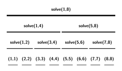
CDQ divide-and-conquer recursion tree

Taking point $8$ as an example, its DP value is updated in solve(1,8), solve(5,8), and solve(7,8). The three sets of points used to update it are the disjoint intervals $(1,4)$ , $(5,6)$ , and $(7,7)$ . Taking point $5$ as another example, its DP value is resolved in solve(1,4), whose update interval is $(1,4)$ . Careful observation shows that the DP value of a point $i$ is updated a number of times equal to $\log$ ; its update intervals are the intervals obtained by splitting $(1,i)$ into $\log$ segments. Therefore, every legal $j$ indeed updates point $i$ , satisfying condition 2.

Next, analyze the execution flow of the algorithm:

The first function to finish is solve(1,1). At this point, the value of $dp_{1}$ has been computed;
The first function to execute a transition is solve(1,2). At this point, the value of $dp_{2}$ has been transitioned;
The second function to finish is solve(2,2). At this point, the value of $dp_{2}$ has been computed;
Next, solve(1,2) finishes, and on interval $(1,2)$ all $dp$ values have been computed;
The next function to execute a transition is solve(1,4). After this transition, the value of $dp_{3}$ has been transitioned;
Next, solve(3,3) finishes. We find that the dp value of $dp_{3}$ has been computed;
Next, the transition executed is solve(3,4). At this point, $dp_{4}$ was transitioned once in solve(1,4) by $(1,2)$ , and is transitioned again by $(3,3)$ , so the value of $dp_{4}$ has also been transitioned;
solve(4,4) finishes, and the value of $dp_{4}$ is complete;
solve(3,4) finishes, and the value of $(3,4)$ is complete;
solve(1,4) finishes, and the value of $(1,4)$ is complete.
……

By simulating the function flow, we find that whenever solve(l,r) ends, all DP values in interval $(l,r)$ have been computed. Since solve(l,mid) has already ended each time we perform a transition, every transition we perform is valid and satisfies condition 1.

In the process above, we find that if the CDQ recursion tree is viewed as a segment tree, CDQ divide and conquer is the in-order traversal function of this segment tree. Thus, we process all DP values in order; only the transition order has been split apart, so the algorithm is correct.

Examples

SDOI2011 Missile Interception

To defend against missile attacks from an enemy country, a country develops a missile interception system. However, the system has a flaw: although its first shell can reach any height and intercept a missile at any speed, every later shell cannot be higher than the previous one, and the flight speed of the intercepted missile cannot exceed that of the previous one. One day, radar detects incoming enemy missiles. Since the system is still in trial operation, there is only one system, so it may be unable to intercept all the missiles.

If all missiles cannot be intercepted, we should of course choose the plan that minimizes the country's losses, namely the plan that intercepts the greatest number of missiles. There may be multiple plans with the maximum number of interceptions; if there are several optimal plans, we randomly choose one as the final interception plan.

Our spies have obtained the height and speed of every enemy missile. Your task is to calculate the probability that each missile is intercepted when the above decision is carried out.

Example code

// A two-dimensional longest increasing subsequence problem
// To determine whether an element can belong to a longest increasing subsequence, run CDQ in both directions
#include <algorithm>
#include <iomanip>
#include <iostream>
using namespace std;
using db = double;
constexpr int N = 1e6 + 10;

struct data_ {
  int h;
  int v;
  int p;
  int ma;
  db ca;
} a[2][N];

int n;
bool tr;

// Rewrite the comparisons below
bool cmp1(const data_& a, const data_& b) {
  if (tr)
    return a.h > b.h;
  else
    return a.h < b.h;
}

bool cmp2(const data_& a, const data_& b) {
  if (tr)
    return a.v > b.v;
  else
    return a.v < b.v;
}

bool cmp3(const data_& a, const data_& b) {
  if (tr)
    return a.p < b.p;
  else
    return a.p > b.p;
}

bool cmp4(const data_& a, const data_& b) { return a.v == b.v; }

struct treearray {
  int ma[2 * N];
  db ca[2 * N];

  void c(int x, int t, db c) {
    for (; x <= n; x += x & (-x)) {
      if (ma[x] == t) {
        ca[x] += c;
      } else if (ma[x] < t) {
        ca[x] = c;
        ma[x] = t;
      }
    }
  }

  void d(int x) {
    for (; x <= n; x += x & (-x)) {
      ma[x] = 0;
      ca[x] = 0;
    }
  }

  void q(int x, int& m, db& c) {
    for (; x > 0; x -= x & (-x)) {
      if (ma[x] == m) {
        c += ca[x];
      } else if (m < ma[x]) {
        c = ca[x];
        m = ma[x];
      }
    }
  }
} ta;

int rk[2][N];

void solve(int l, int r, int t) {  // recursive traversal
  if (r - l == 1) {
    return;
  }
  int mid = (l + r) / 2;
  solve(l, mid, t);
  sort(a[t] + mid + 1, a[t] + r + 1, cmp1);
  int p = l + 1;
  for (int i = mid + 1; i <= r; i++) {
    for (; (cmp1(a[t][p], a[t][i]) || a[t][p].h == a[t][i].h) && p <= mid;
         p++) {
      ta.c(a[t][p].v, a[t][p].ma, a[t][p].ca);
    }
    db c = 0;
    int m = 0;
    ta.q(a[t][i].v, m, c);
    if (a[t][i].ma < m + 1) {
      a[t][i].ma = m + 1;
      a[t][i].ca = c;
    } else if (a[t][i].ma == m + 1) {
      a[t][i].ca += c;
    }
  }
  for (int i = l + 1; i <= mid; i++) {
    ta.d(a[t][i].v);
  }
  sort(a[t] + mid, a[t] + r + 1, cmp3);
  solve(mid, r, t);
  sort(a[t] + l + 1, a[t] + r + 1, cmp1);
}

void ih(int t) {
  sort(a[t] + 1, a[t] + n + 1, cmp2);
  rk[t][1] = 1;
  for (int i = 2; i <= n; i++) {
    rk[t][i] = (cmp4(a[t][i], a[t][i - 1])) ? rk[t][i - 1] : i;
  }
  for (int i = 1; i <= n; i++) {
    a[t][i].v = rk[t][i];
  }
  sort(a[t] + 1, a[t] + n + 1, cmp3);
  for (int i = 1; i <= n; i++) {
    a[t][i].ma = 1;
    a[t][i].ca = 1;
  }
}

int len;
db ans;

int main() {
  cin.tie(nullptr)->sync_with_stdio(false);
  cin >> n;
  for (int i = 1; i <= n; i++) {
    cin >> a[0][i].h >> a[0][i].v;
    a[0][i].p = i;
    a[1][i].h = a[0][i].h;
    a[1][i].v = a[0][i].v;
    a[1][i].p = i;
  }
  ih(0);
  solve(0, n, 0);
  tr = true;
  ih(1);
  solve(0, n, 1);
  tr = true;
  sort(a[0] + 1, a[0] + n + 1, cmp3);
  sort(a[1] + 1, a[1] + n + 1, cmp3);
  for (int i = 1; i <= n; i++) {
    len = max(len, a[0][i].ma);
  }
  cout << len << '\n';
  for (int i = 1; i <= n; i++) {
    if (a[0][i].ma == len) {
      ans += a[0][i].ca;
    }
  }
  cout << fixed << setprecision(5);
  for (int i = 1; i <= n; i++) {
    if (a[0][i].ma + a[1][i].ma - 1 == len) {
      cout << (a[0][i].ca * a[1][i].ca) / ans << ' ';
    } else {
      cout << "0.00000 ";
    }
  }
  return 0;
}

Turning dynamic problems into static problems

In the first two cases, CDQ divide and conquer halves the sequence and recursively processes point-pair relations to obtain good complexity. In this section, however, it is the time sequence that is halved, rather than an ordinary sequence.

This applies to data-structure problems that need to support “perform xxx updates and then xxx queries.” Such problems have two characteristics:

If the queries are offline, all operations naturally form a sequence in time order.
Every update is closely related to subsequent queries. There are $O(n^2)$ such “update–query” relationships.

We can apply CDQ divide and conquer to this sequence of operations, processing the relationships between updates and queries.

Similar to CDQ divide and conquer for point-pair relations, suppose the sequence being divided is $(l,r)$ . We first recursively process the update–query relationships between $(l,mid)$ and $(mid,r)$ , and then process all update–query relationships with $l \leq i \leq mid$ and $mid+1 \leq j \leq r$ , where $i$ is an update and $j$ is a query.

If the updates are independent, we do not need to process the temporal relationship between $l \leq i \leq mid$ and $mid+1 \leq j \leq r$ , or between solve(l,mid) and solve(mid+1,r) (as in ordinary addition and subtraction problems). However, if the updates are not independent (for example, assignments), the state of the sequence after an update may depend on the previous sequence. In that case, the step that processes all update–query relationships crossing mid must be placed between solve(l,mid) and solve(mid+1,r). The reason is the same as for CDQ divide-and-conquer optimization of 1D/1D dynamic programming: dividing according to in-order traversal is necessary to ensure that every update is executed strictly in time order.

Examples

Rectangle addition and rectangle sum

Maintain a two-dimensional array, support adding a number to a rectangular region, and answer the sum of a rectangular region on each query.

Solution idea

For the version without updates, namely “given a two-dimensional array and answer multiple queries for the sum of a rectangular region,” a classic scanline plus segment-tree approach is available. Specifically, split each rectangle into an insertion and a deletion, split each query into a difference of two-dimensional prefix sums, and finally process everything offline. However, the original problem includes updates, so this method cannot be used directly.

Try applying CDQ divide and conquer. We process all queries and updates offline. These operations form a sequence with $O(N^2)$ update–query relationships. We still use the general CDQ process, divide all relationships into three categories, handle only the relationships crossing $mid$ at this level, and solve the remaining relationships recursively.

We find that all updates have already been completed before the queries. The original problem is therefore equivalent to “there are some static rectangles on a plane, and we repeatedly query the sum of a rectangular region.”

Use a scanline in $O(n\log n)$ time to process all update–query relationships crossing $mid$ ; the remaining task is to recursively divide and conquer the relationships on the left and right.

In this CDQ divide and conquer, the same query is processed $O(\log n)$ times. This is harmless because the updates contributing to a given query are disjoint. The overall time complexity is $T(n)=T(\lfloor \frac{n}{2} \rfloor)+T(\lceil \frac{n}{2} \rceil)+ O(n\log n)=O(n\log^2n)$ .

Observing the algorithm above, we find that at first we can solve only the static rectangle-addition and rectangle-sum problem. By simply applying CDQ divide and conquer, however, we can solve a dynamic version offline. The essence of turning a dynamic problem into a static one is that CDQ divide and conquer processes only update–query relationships crossing a chosen point at each step, so we need only consider the simple case where all queries occur after the updates. This is why CDQ divide and conquer is called a “tool for turning dynamic problems into static problems.”

[Ynoi2016] Insects in the Mirror

Maintain a sequence of length $n$ , denoted $a_i$ , with $m$ operations.

Set the value on interval $[l,r]$ to $x$ ;
Query how many distinct values appear in interval $[l,r]$ , counting a value only once even if it appears multiple times.

In one sentence: range assignment and range color counting.

Solution idea

Maintain the position of the first point to the left of each position with the same color, denoted $pre_{i}$ . The range color-counting problem is then transformed into a classic two-dimensional counting problem.

By treating each consecutive color segment as a point, we can prove that the total change in $pre$ is $O(n+m)$ : each operation changes only $O(1)$ values of $pre$ . Thus, CDQ divide and conquer can solve the dynamic point-addition and rectangle-sum problem.

The concrete changes to the $pre$ array can be handled with std::set. This technique of using a set to maintain consecutive intervals is also called an old driver tree.

Example code

#include <algorithm>
#include <iostream>
#include <map>
#include <set>
#define SNI set<nod>::iterator
#define SDI set<data>::iterator
using namespace std;
constexpr int N = 1e5 + 10;
int n;
int m;
int pre[N];
int npre[N];
int a[N];
int tp[N];
int lf[N];
int rt[N];
int co[N];

struct modi {
  int t;
  int pos;
  int pre;
  int va;

  friend bool operator<(modi a, modi b) { return a.pre < b.pre; }
} md[10 * N];

int tp1;

struct qry {
  int t;
  int l;
  int r;
  int ans;

  friend bool operator<(qry a, qry b) { return a.l < b.l; }
} qr[N];

int tp2;
int cnt;

bool cmp(const qry& a, const qry& b) { return a.t < b.t; }

void modify(int pos, int co)  // modification function
{
  if (npre[pos] == co) return;
  md[++tp1] = modi{++cnt, pos, npre[pos], -1};
  md[++tp1] = modi{++cnt, pos, npre[pos] = co, 1};
}

namespace prew {
int lst[2 * N];
map<int, int> mp;  // discretize in advance

void prew() {
  cin.tie(nullptr)->sync_with_stdio(false);
  cin >> n >> m;
  for (int i = 1; i <= n; i++) cin >> a[i], mp[a[i]] = 1;
  for (int i = 1; i <= m; i++) {
    cin >> tp[i] >> lf[i] >> rt[i];
    if (tp[i] == 1) cin >> co[i], mp[co[i]] = 1;
  }
  map<int, int>::iterator it, it1;
  for (it = mp.begin(), it1 = it, ++it1; it1 != mp.end(); ++it, ++it1)
    it1->second += it->second;
  for (int i = 1; i <= n; i++) a[i] = mp[a[i]];
  for (int i = 1; i <= n; i++)
    if (tp[i] == 1) co[i] = mp[co[i]];
  for (int i = 1; i <= n; i++) pre[i] = lst[a[i]], lst[a[i]] = i;
  for (int i = 1; i <= n; i++) npre[i] = pre[i];
}
}  // namespace prew

namespace colist {
struct data {
  int l;
  int r;
  int x;

  friend bool operator<(data a, data b) { return a.r < b.r; }
};

set<data> s;

struct nod {
  int l;
  int r;

  friend bool operator<(nod a, nod b) { return a.r < b.r; }
};

set<nod> c[2 * N];
set<int> bd;

void split(int mid) {  // split one node into two nodes
  SDI it = s.lower_bound(data{0, mid, 0});
  data p = *it;
  if (mid == p.r) return;
  s.erase(p);
  s.insert(data{p.l, mid, p.x});
  s.insert(data{mid + 1, p.r, p.x});
  c[p.x].erase(nod{p.l, p.r});
  c[p.x].insert(nod{p.l, mid});
  c[p.x].insert(nod{mid + 1, p.r});
}

void del(set<data>::iterator it) {  // delete an iterator
  bd.insert(it->l);
  SNI it1, it2;
  it1 = it2 = c[it->x].find(nod{it->l, it->r});
  ++it2;
  if (it2 != c[it->x].end()) bd.insert(it2->l);
  c[it->x].erase(it1);
  s.erase(it);
}

void ins(data p) {  // insert a node
  s.insert(p);
  SNI it = c[p.x].insert(nod{p.l, p.r}).first;
  ++it;
  if (it != c[p.x].end()) {
    bd.insert(it->l);
  }
}

void stv(int l, int r, int x) {  // range assignment
  if (l != 1) split(l - 1);
  split(r);
  int p = l;  // after splitting twice, delete all intervals
  while (p != r + 1) {
    SDI it = s.lower_bound(data{0, p, 0});
    p = it->r + 1;
    del(it);
  }
  ins(data{l, r, x});  // scan the set to process all changes to pre values
  for (set<int>::iterator it = bd.begin(); it != bd.end(); ++it) {
    SDI it1 = s.lower_bound(data{0, *it, 0});
    if (*it != it1->l)
      modify(*it, *it - 1);
    else {
      SNI it2 = c[it1->x].lower_bound(nod{0, *it});
      if (it2 != c[it1->x].begin())
        --it2, modify(*it, it2->r);
      else
        modify(*it, 0);
    }
  }
  bd.clear();
}

void ih() {
  int nc = a[1];
  int ccnt = 1;  // insert a consecutive segment into the set
  for (int i = 2; i <= n; i++)
    if (nc != a[i]) {
      s.insert(data{i - ccnt, i - 1, nc}), c[nc].insert(nod{i - ccnt, i - 1});
      nc = a[i];
      ccnt = 1;
    } else {
      ccnt++;
    }
  s.insert(data{n - ccnt + 1, n, a[n]}), c[a[n]].insert(nod{n - ccnt + 1, n});
}
}  // namespace colist

namespace CDQ {
struct treearray  // Fenwick tree
{
  int ta[N];

  void c(int x, int t) {
    for (; x <= n; x += x & (-x)) ta[x] += t;
  }

  void d(int x) {
    for (; x <= n; x += x & (-x)) ta[x] = 0;
  }

  int q(int x) {
    int r = 0;
    for (; x; x -= x & (-x)) r += ta[x];
    return r;
  }

  void clear() {
    for (int i = 1; i <= n; i++) ta[i] = 0;
  }
} ta;

int srt[N];

bool cmp1(const int& a, const int& b) { return pre[a] < pre[b]; }

void solve(int l1, int r1, int l2, int r2, int L, int R) {  // CDQ
  if (l1 == r1 || l2 == r2) return;
  int mid = (L + R) / 2;
  int mid1 = l1;
  while (mid1 != r1 && md[mid1 + 1].t <= mid) mid1++;
  int mid2 = l2;
  while (mid2 != r2 && qr[mid2 + 1].t <= mid) mid2++;
  solve(l1, mid1, l2, mid2, L, mid);
  solve(mid1, r1, mid2, r2, mid, R);
  if (l1 != mid1 && mid2 != r2) {
    sort(md + l1 + 1, md + mid1 + 1);
    sort(qr + mid2 + 1, qr + r2 + 1);
    for (int i = mid2 + 1, j = l1 + 1; i <= r2; i++) {  // consider the contribution from the left to the right
      while (j <= mid1 && md[j].pre < qr[i].l) ta.c(md[j].pos, md[j].va), j++;
      qr[i].ans += ta.q(qr[i].r) - ta.q(qr[i].l - 1);
    }
    for (int i = l1 + 1; i <= mid1; i++) ta.d(md[i].pos);
  }
}

void mainsolve() {
  colist::ih();
  for (int i = 1; i <= m; i++)
    if (tp[i] == 1)
      colist::stv(lf[i], rt[i], co[i]);
    else
      qr[++tp2] = qry{++cnt, lf[i], rt[i], 0};
  sort(qr + 1, qr + tp2 + 1);
  for (int i = 1; i <= n; i++) srt[i] = i;
  sort(srt + 1, srt + n + 1, cmp1);
  for (int i = 1, j = 1; i <= tp2; i++) {  // initialize each query's value
    while (j <= n && pre[srt[j]] < qr[i].l) ta.c(srt[j], 1), j++;
    qr[i].ans += ta.q(qr[i].r) - ta.q(qr[i].l - 1);
  }
  ta.clear();
  sort(qr + 1, qr + tp2 + 1, cmp);
  solve(0, tp1, 0, tp2, 0, cnt);
  sort(qr + 1, qr + tp2 + 1, cmp);
  for (int i = 1; i <= tp2; i++) cout << qr[i].ans << '\n';
}
}  // namespace CDQ

int main() {
  prew::prew();
  CDQ::mainsolve();
  return 0;
}

[HNOI2010] City Construction

PS Country is a large country with many cities. King Louis has racked his brains over the country's transportation infrastructure. Louis can build roads between some cities, and building roads between different pairs of cities incurs different costs.

Louis wants to build the fewest roads needed to connect all cities in the country. However, due to various factors, the cost of building roads between cities changes over time. Louis continually receives messages that the cost of a road has changed, and wants to know the minimum total cost that connects all cities immediately after each message. Louis asks you to complete this task.

In one sentence: given a graph with dynamically changing edge weights, output the minimum cost of a minimum spanning tree after each edge-weight update.

Solution idea

In fact, a segment-tree divide and conquer combined with an LCT can solve this problem, but its constant factor is too large and passing may require delicate constant-factor optimizations. It is therefore worth considering CDQ divide and conquer instead.

Unlike ordinary problems solved by CDQ divide and conquer, there is no update–query relationship here to guide the divide and conquer, because we cannot consider independently what contribution “updating one edge makes to the minimum spanning tree of the whole graph.” The traditional CDQ idea does not seem to work well.

The previous example shows that ordinary CDQ divide and conquer has a special relationship with segment trees: during CDQ we implicitly build a segment tree (because the CDQ recursion tree is a segment tree). Ordinary CDQ considers the relationship between the left and right children of a segment tree. For this problem, however, we need to consider the relationship between a parent and its children; in other words, when we are in the interval $solve(l,r)$ , if we can make the graph size depend on the interval length, we can solve the problem.

So how should we design the algorithm concretely?

Suppose we are constructing the edge set of the minimum spanning tree for interval $(l,r)$ and know the edge set of its parent minimum spanning tree. We assign the changing edges in interval $(l,r)$ weights of $+ \infty$ and $-\infty$ respectively, run Kruskal once for each, and find the edges that belong to the minimum spanning tree.

For an edge:

If every modified edge in the minimum spanning tree is assigned weight $+\infty$ and the edge does not appear in the tree, it cannot appear in the minimum spanning tree of the queries in $(l,r)$ . Therefore, we add only minimum-spanning-tree edges to the edge set of $(l,r)$ .
If every modified edge in the minimum spanning tree is assigned weight $-\infty$ and the edge appears in the tree, it must appear in the minimum spanning tree for interval $(l,r)$ . We can then use a disjoint-set union to contract the corresponding vertices and add the weights of these edges to the answer.

This constructs the edge set for interval $(l,r)$ . The minimum spanning tree computed from these edges is equivalent to the minimum spanning tree computed directly from the original graph.

Why, then, is the complexity correct?

First, every modified edge is added to our edge set, and there are $O(len)$ such edges.

Next, we need to prove that the edge set does not contain too many unmodified edges. We add only tree edges from the minimum spanning tree in which all edge weights are $+\infty$ , so the number of edges we add does not exceed the number of vertices in the current graph.

We now only need to prove that the number of vertices in each recursive-level graph is $O(len)$ , which implies that the number of edges is $O(len)$ .

Proving that the number of vertices is within a constant factor of $O(len)$ is straightforward. Each time we recurse downward, the contracted edges are unmodified edges appearing in the $-\infty$ spanning tree; equivalently, we cut all modified edges appearing in the $-\infty$ spanning tree. We can cut at most $len$ edges, so the graph splits into at most $O(len)$ connected components. Thus the new graph has $O(len)$ vertices. Therefore, each graph on which we run Kruskal has $O(len)$ edges, and the time complexity of each level is $O(n\log n)$ .

The time complexity is $T(n)=T(\lfloor \frac{n}{2} \rfloor)+T(\lceil \frac{n}{2} \rceil)+ O(n\log n)=O(n\log^2n)$ .

The implementation may be somewhat difficult. Note that the disjoint-set union cannot use path compression, or rollback operations will no longer be supported. When contracting vertices, there is no need to perform the contraction physically; each level's Kruskal can operate directly on the disjoint-set union from the previous level.

Example code

#include <algorithm>
#include <iostream>
#include <stack>
#include <vector>
using namespace std;
using ll = long long;
int n;
int m;
int ask;

struct bcj {
  int fa[20010];
  int size[20010];

  struct opt {
    int u;
    int v;
  };

  stack<opt> st;

  void ih() {
    for (int i = 1; i <= n; i++) fa[i] = i, size[i] = 1;
  }

  int f(int x) { return (fa[x] == x) ? x : f(fa[x]); }

  void u(int x, int y) {  // With rollback
    int u = f(x);
    int v = f(y);
    if (u == v) return;
    if (size[u] < size[v]) swap(u, v);
    size[u] += size[v];
    fa[v] = u;
    opt o;
    o.u = u;
    o.v = v;
    st.push(o);
  }

  void undo() {
    opt o = st.top();
    st.pop();
    fa[o.v] = o.v;
    size[o.u] -= size[o.v];
  }

  void clear(int tim) {
    while (st.size() > tim) {
      undo();
    }
  }
} s, s1;

struct edge  // Static edge
{
  int u;
  int v;
  ll val;
  int mrk;

  friend bool operator<(edge a, edge b) { return a.val < b.val; }
} e[50010];

struct moved {
  int u;
  int v;
};  // Dynamic edge

struct query {
  int num;
  ll val;
  ll ans;
} q[50010];

bool book[50010];  // Query
vector<edge> ve[30];
vector<moved> vq;
vector<edge> tr;
ll res[30];
int tim[30];

void pushdown(int dep)  // Contract edges
{
  tr.clear();  // Make a copy here so that the operations can be rolled back
  for (int i = 0; i < ve[dep].size(); i++) {
    tr.push_back(ve[dep][i]);
  }
  sort(tr.begin(), tr.end());
  for (int i = 0; i < tr.size(); i++) {  // Useless edges
    if (s1.f(tr[i].u) == s1.f(tr[i].v)) {
      tr[i].mrk = -1;
      continue;
    }
    s1.u(tr[i].u, tr[i].v);
  }
  s1.clear(0);
  res[dep + 1] = res[dep];
  for (int i = 0; i < vq.size(); i++) {
    s1.u(vq[i].u, vq[i].v);
  }
  vq.clear();
  for (int i = 0; i < tr.size(); i++) {  // Mandatory edges
    if (tr[i].mrk == -1 || s1.f(tr[i].u) == s1.f(tr[i].v)) continue;
    tr[i].mrk = 1;
    s1.u(tr[i].u, tr[i].v);
    s.u(tr[i].u, tr[i].v);
    res[dep + 1] += tr[i].val;
  }
  s1.clear(0);
  ve[dep + 1].clear();
  for (int i = 0; i < tr.size(); i++) {  // Contract edges
    if (tr[i].mrk != 0) continue;
    edge p;
    p.u = s.f(tr[i].u);
    p.v = s.f(tr[i].v);
    if (p.u == p.v) continue;
    p.val = tr[i].val;
    p.mrk = 0;
    ve[dep + 1].push_back(p);
  }
  return;
}

void solve(int l, int r, int dep) {
  tim[dep] = s.st.size();
  int mid = (l + r) / 2;
  if (r - l == 1) {  // Termination condition
    edge p;
    p.u = s.f(e[q[r].num].u);
    p.v = s.f(e[q[r].num].v);
    p.val = q[r].val;
    e[q[r].num].val = q[r].val;
    p.mrk = 0;
    ve[dep].push_back(p);
    pushdown(dep);
    q[r].ans = res[dep + 1];
    s.clear(tim[dep - 1]);
    return;
  }
  for (int i = l + 1; i <= mid; i++) {
    book[q[i].num] = true;
  }
  for (int i = mid + 1; i <= r; i++) {  // Dynamic to static
    if (book[q[i].num]) continue;
    edge p;
    p.u = s.f(e[q[i].num].u);
    p.v = s.f(e[q[i].num].v);
    p.val = e[q[i].num].val;
    p.mrk = 0;
    ve[dep].push_back(p);
  }
  for (int i = l + 1; i <= mid; i++) {  // Query to dynamic
    moved p;
    p.u = s.f(e[q[i].num].u);
    p.v = s.f(e[q[i].num].v);
    vq.push_back(p);
  }
  pushdown(dep);  // The following operations are rolled back
  for (int i = mid + 1; i <= r; i++) {
    if (book[q[i].num]) continue;
    ve[dep].pop_back();
  }
  for (int i = l + 1; i <= mid; i++) {
    book[q[i].num] = false;
  }
  solve(l, mid, dep + 1);
  for (int i = 0; i < ve[dep].size(); i++) {
    ve[dep][i].mrk = 0;
  }
  for (int i = mid + 1; i <= r; i++) {
    book[q[i].num] = true;
  }
  for (int i = l + 1; i <= mid; i++) {  // Dynamic to static
    if (book[q[i].num]) continue;
    edge p;
    p.u = s.f(e[q[i].num].u);
    p.v = s.f(e[q[i].num].v);
    p.val = e[q[i].num].val;
    p.mrk = 0;
    ve[dep].push_back(p);
  }
  for (int i = mid + 1; i <= r; i++) {  // Query to dynamic
    book[q[i].num] = false;
    moved p;
    p.u = s.f(e[q[i].num].u);
    p.v = s.f(e[q[i].num].v);
    vq.push_back(p);
  }
  pushdown(dep);
  solve(mid, r, dep + 1);
  s.clear(tim[dep - 1]);
  return;  // Roll time back to the previous level
}

int main() {
  cin.tie(nullptr)->sync_with_stdio(false);
  cin >> n >> m >> ask;
  s.ih();
  s1.ih();
  for (int i = 1; i <= m; i++) {
    cin >> e[i].u >> e[i].v >> e[i].val;
  }
  for (int i = 1; i <= ask; i++) {
    cin >> q[i].num >> q[i].val;
  }
  for (int i = 1; i <= ask; i++) {  // Initially dynamic edges
    book[q[i].num] = true;
    moved p;
    p.u = e[q[i].num].u;
    p.v = e[q[i].num].v;
    vq.push_back(p);
  }
  for (int i = 1; i <= m; i++) {  // Initially static
    if (book[i]) continue;
    ve[1].push_back(e[i]);
  }
  for (int i = 1; i <= ask; i++) {
    book[q[i].num] = false;
  }
  solve(0, ask, 1);
  for (int i = 1; i <= ask; i++) {
    cout << q[i].ans << '\n';
  }
  return 0;
}

References and notes

Footnotes

A discussion of a divide-and-conquer algorithm from "Cash" ↩