Finite State Machine

Prerequisite knowledge: Language and decision problems

Finite State Machine (Finite State Machine, FSM, also abbreviated as an automaton below) is the simplest class of computational models, characterized by extremely limited descriptive power and resources. Automata are widely used in OI and computer science, and their ideas appear in many string algorithms, so it is recommended to learn automata before studying string algorithms such as KMP, the Aho–Corasick automaton, and SAM.

Introduction to Automata

First, let us understand what automata are used for: an automaton is a mathematical model for determining whether a signal sequence satisfies a particular pattern or rule.

Some of the terms in this sentence can be explained more concretely. A “signal sequence” is a sequence of signals arranged in order, such as each character of a string from beginning to end, each number of an array from $1$ to $n$, or each digit of a number from most significant to least significant. “Determining whether a rule is satisfied” can be understood as asking whether we care about the sequence belonging to a particular set. This set is defined by rules that we specify in advance, such as “all binary strings of even length” or “all palindromes.”

Sometimes we need to answer questions of this kind: does a given sequence have a certain property? For example, is a binary number odd, is a string a palindrome, or is it a subsequence of another string? An automaton is a mathematical tool for solving such questions.

The way an automaton works is very similar to a flowchart. Suppose you want to order a cup of milk tea on a food-delivery platform; all your choices form a sequence. The following flowchart is an example:

For example, if your sequence of choices is “open the ordering interface -> choose milk tea -> have enough money for the milk tea,” then the states you pass through in order might be “food-delivery platform -> ordering interface -> pay for the milk tea -> bought the milk tea.” In this way, our “milk-tea automaton” determines, based on our choices, whether we bought the milk tea. We can also see that there may be more than one way to reach a state. Likewise, if you did not buy the milk tea, you might have exited directly from the ordering interface, or you might not have had enough money and therefore failed to buy it.

Using this automaton, we divided signal sequences into two classes: signal sequences that bought the milk tea and signal sequences that did not. By looking at the final state, we completed a decision problem.

Although we just used a flowchart as an analogy for how an automaton works, the flowchart itself is only an intuitive visualization tool and does not constitute the mathematical definition of an automaton. To characterize the structure of an automaton more precisely, we need to abstract the elements of the flowchart. After abstraction, we find that the structure of the flowchart can actually be simplified to a directed graph, where each vertex represents a state and each directed edge represents a transition between states.

Thus, the core structure of an automaton can be formally viewed as a directed graph, which we call a state graph.

An automaton works similarly to a flowchart, with the following differences: every vertex of an automaton is a decision vertex; a vertex of an automaton is just a state, not a task; and an edge of an automaton can accept multiple characters (not limited to T or F).

For example, the automaton for “determining whether a binary number is even” is as follows:

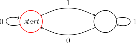
Starting from the initial vertex, accept the binary sequence of the number from the most significant digit to the least significant digit, and then see where you end up. If you end at a red-circled vertex, the number is even; otherwise, it is not.

Here, we should emphasize that we will repeatedly use terms such as “character” and “character set” below. This does not mean that automata can only be applied in the string domain: a character need not be a letter such as $\tt abc\cdots z$; it may also represent a choice.

If we need to determine the relationship between one finite signal sequence and another signal sequence (for example, whether the other signal sequence is a subsequence of a signal sequence), a common method is to construct an automaton for that finite signal sequence. This will be discussed when learning KMP.

Note that an automaton is only a mathematical model, and is neither an algorithm nor a data structure. There are many ways to implement the same automaton, and they may have different time and space complexities.

Next, you can either continue studying automata on this page, or learn concrete examples such as KMP, the Aho–Corasick automaton, or SAM.

FSMs are divided into two categories: deterministic finite automata and nondeterministic finite automata.

Deterministic Finite Automata

A deterministic finite automaton (Deterministic Finite Automaton, DFA) is characterized by a deterministic decision process. Taking the “milk-tea automaton” as an example, as soon as you open the ordering interface, you enter the ordering interface; unexpected events such as a network crash preventing it from opening or a dead phone screen do not occur.

A DFA can be represented simply by the following structure:

// Deterministic Finite Automaton (DFA)
struct DFA {
  int m;                                // Alphabet size.
  int n;                                // Number of states.
  int q0;                               // Initial state.
  std::vector<std::vector<int>> trans;  // Transitions: trans[c][q].
  std::vector<int> acc;                 // Acceptance labels per state:
                                        // - 0 = non-accepting

  DFA(int m, int n = 0, int q0 = 0)
      : m(m), n(n), q0(q0), trans(m, std::vector<int>(n)), acc(n) {}

  // Returns minimized DFA via Hopcroft's algorithm.
  DFA hopcroft_minimize() const;
};

The process of finding the state sequence of an input string $w$ in a DFA and determining whether it is accepted is called computation.

When a DFA reads a string, it transitions one character at a time from the initial state according to the transition function. If, after reading all characters of a string, it is in an accepting state, we say that the DFA accepts the string; otherwise, we say that the DFA rejects the string.

Not every language can be recognized by a DFA.

As mentioned above, an automaton can be represented by a state graph. The following is a DFA that accepts exactly the strings $\tt a$, $\tt ab$, and $\tt aac$:

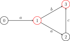
(The dead state is omitted from the figure; all transitions not shown point to that dead state.)

Nondeterministic Finite Automata

A nondeterministic finite automaton¹ (Nondeterministic Finite Automaton, NFA) is a natural generalization of a DFA. In an NFA, for any state and any character, there may be zero, one, or multiple successor states. At the same time, the NFA discussed in this section allows epsilon transitions, meaning that a state can transition to one of its successors without consuming any character.

For example, consider the “milk-tea automaton” again. After placing the order, even if you have enough money for the milk tea, poor network conditions may cause you not to buy it; this gives multiple successors. It is also possible that, because you were slow, the input string (that is, the sequence of operations) is the same but the milk tea has sold out, so you do not buy it; this is the presence of an epsilon transition, which may or may not be taken. The above automaton can be modified slightly to implement this behavior:

Clearly, every DFA is an NFA, so an NFA can recognize at least all regular languages. But as an extension of a DFA, can an NFA recognize more languages? In fact, it cannot; we will discuss the equivalence of DFAs and NFAs later.

The computation of an NFA is equivalent to running multiple DFAs simultaneously. At each step, all possibilities are enumerated; finally, as long as one branch reaches an accepting state, the NFA accepts the entire string.

Because epsilon transitions are allowed, when representing $w$ as $y_1y_2\cdots y_m\in\Sigma^*_\varepsilon$, any number of epsilon symbols may be inserted. For example, the string $\mathtt{abc}$ can be represented as $\mathtt{a}\varepsilon\mathtt{bc}\varepsilon\varepsilon\in\Sigma^*_\varepsilon$. Unlike a DFA, where each input corresponds to only one result, each input to an NFA may correspond to multiple results, forming a set of results.

Equivalence of DFAs and NFAs

We call two automata equivalent if and only if they recognize the same language. DFAs and NFAs are equivalent, meaning that every NFA is equivalent to some DFA; therefore, the class of languages recognized by NFAs is also the class of all regular languages. Every DFA can be directly viewed as an NFA; conversely, an NFA can be converted into a DFA using powerset construction.

Although NFAs and DFAs have the same language-recognition power, NFAs are still useful. This is because, for some regular languages, an NFA requires far fewer states than a DFA. For example, one can construct an NFA with $n$ states whose corresponding minimal DFA has $\Theta(2^n)$ states. In this case, directly computing the NFA has better time complexity.

Time Complexity of Computing DFAs and NFAs

Suppose the given string has length $n$, the automaton has $s$ states, and the alphabet size is constant. Then, clearly, the time complexity of DFA computation is $O(n)$; we only need to simulate the process above.

The time complexity of naive NFA computation is $O(ns^2)$, because we need to consider every possible successor and the complexity required to merge states. Of course, bitsets or the Method of Four Russians can be used to optimize the computation to $O\left(\dfrac{ns^2}{w}\right)$ or $O\left(\dfrac{ns^2}{w\cdot \log n}\right)$.

Regular Expressions and Regular Languages

This section discusses the definitions and properties of regular expressions and regular languages, and examines the relationship between regular expressions and FSMs.

Regular Expressions

A regular expression is another commonly used way to describe regular languages. Although we can see this name in many modern languages (such as Python), those languages actually implement a superset of regular expressions.

The goal of a regular expression is to describe a language using these symbols. Every regular expression has a corresponding formal language.

Of course, once the precedence of the operations has been specified, these parentheses can be omitted when doing so causes no ambiguity.

Every regular expression can be converted into an NFA through Thompson's construction, and every DFA can be converted into a regular expression through the State Elimination Method². Therefore, regular expressions and FSMs are equivalent.

Regular Languages

In this subsection, rather than considering particular regular expressions, we consider regular expressions parameterized by variables (where the variables may be arbitrary regular languages). Applying the algebraic laws of regular expressions helps simplify regular expressions.

The closure properties of regular languages are also important. These properties allow us to start from some simple automata and, through certain operations, construct finite-state machines (FSMs) that recognize other languages. In short, closure properties can serve as tools for constructing complex FSMs.

For the closure properties of regular languages, we have:

A simple consequence is that every finite language is regular. In fact, a Trie is an automaton that recognizes it.

Myhill–Nerode Theorem

The Myhill–Nerode theorem provides a criterion for determining whether a language is regular. It describes the structural properties of regular languages through the concept of equivalence classes.

In other words, if, for two strings $x$ and $y$, after appending the same arbitrary string $z$ (including the empty string) to $x$ and $y$, they are always either both in $L$ or both not in $L$, then we say that $x$ and $y$ are equivalent with respect to $L$.

According to the definition above, we partition the set of all finite strings into one or more equivalence classes. If and only if the number of these equivalence classes is finite, we can use them to construct a DFA that recognizes the language. The number of states of this DFA equals the number of equivalence classes. Moreover, this number of states is the smallest among all DFAs that can recognize the language. This is the Myhill–Nerode theorem.

This theorem provides a way to construct a DFA using an equivalence relation:

• The state set consists of all equivalence classes obtained from the partition induced by the equivalence relation. Choose any representative string for each equivalence class (for example, a shortest string).
• To construct the transition function, append the transition character to the chosen representative string and find the state corresponding to the equivalence class containing the resulting string; this is the successor state of the transition. Since all strings in the same equivalence class are equivalent, the choice of representative string does not affect the transition result.
• The initial state is the equivalence class corresponding to the empty string $\varepsilon$.
• The accepting state set is the set of equivalence classes whose representative strings belong to the given language.

As a classic example, a suffix automaton is a minimal DFA constructed using the Myhill–Nerode theorem.

The Myhill–Nerode theorem is usually applied to construct a DFA for an infinite regular language. In many cases, the problem conditions are simple enough that we need only examine the set of strings whose lengths are not too large, and can then construct an automaton recognizing the entire language.

Example Problem

This section introduces the practical application of the Myhill–Nerode theorem through an example problem.

#include <array>
#include <iostream>
#include <unordered_map>
#include <vector>

constexpr int L = 3;
std::array<int, 1 << L> op;
constexpr int X = (1 << L) - 2;

// Build a DFA that accepts binary strings which evaluate to a given string.
//   0b000 → "00"
//   0b001 → "01"
//   0b010 → "10"
//   0b011 → "11"
//   0b100 → "0"
//   0b101 → "1"
DFA build(int x) {
  constexpr int L1 = 9, L2 = 6;
  // The result for string `st` of length `len` is stored at (1 << len) | st.
  const auto idx = [](int len, int st) -> int { return (1 << len) | st; };

  // Compute which bit strings are accepted using dynamic programming.
  std::vector<bool> acc(1 << (L1 + L2 + 1));
  acc[(x >> 2) ? idx(1, x & 1) : idx(2, x)] = true;

  for (int len = (x >> 2) ? 3 : 4; len <= L1 + L2; len += 2) {
    for (int st = 0; st < (1 << len); ++st) {
      for (int i = 0; i + L <= len; ++i) {
        // Replace st[i..i+2] using the op[] rule, and check if the result is
        // accepted. Result = st[0..i-1] + op[st[i..i+2]] + st[i+3..end]
        int pr =
            ((((st >> (i + L)) << 1) | op[(st >> i) & ((1 << L) - 1)]) << i) |
            (st & ((1 << i) - 1));
        if (acc[idx(len - 2, pr)]) {
          acc[idx(len, st)] = true;
          break;
        }
      }
    }
  }

  // Construct a DFA using the Myhill-Nerode theorem.
  DFA dfa(2);
  std::unordered_map<std::vector<bool>, int>
      mp;                // Maps characteristic vectors to state IDs.
  std::vector<int> sts;  // Representative 01 strings for each state.
  std::vector<int> ids(1 << (L1 + 1));  // Maps 01 strings to DFA state IDs.

  for (int len = 0; len <= L1; ++len) {
    for (int st = (1 << len); st < (2 << len); ++st) {
      // Construct characteristic vector for this prefix.
      std::vector<bool> key(1 << (L2 + 1));
      for (int nxt = 0; nxt <= L2; ++nxt)
        std::copy(acc.begin() + (st << nxt), acc.begin() + ((st + 1) << nxt),
                  key.begin() + (1 << nxt));
      if (!mp.count(key)) {
        mp[key] = dfa.n++;
        sts.push_back(st);
        dfa.acc.push_back(key[idx(0, 0)]);
      }
      ids[st] = mp[key];
    }
  }

  // Build transitions.
  for (int c = 0; c < 2; ++c) {
    dfa.trans[c].resize(dfa.n);
    for (int i = 0; i < dfa.n; ++i) dfa.trans[c][i] = ids[(sts[i] << 1) | c];
  }

  return dfa;
}

std::vector<DFA> dfa;

// Initialize the DFA's.
void init() {
  std::string s;
  std::cin >> s;
  for (int i = 0; i < (1 << L); ++i) op[i] = s[i] - '0';
  std::swap(op[1], op[4]);
  std::swap(op[3], op[6]);
  for (int x = 0; x < X; ++x) dfa.push_back(build(x));
}

std::string s;
constexpr int B = 5;  // Block size is 2^B.
std::vector<std::vector<std::array<std::vector<int>, X>>> pre;

void precompute() {
  int n = s.size();
  for (int i = 0; i < n; ++i) s[i] -= '0';
  int nn = ((n - 1) >> B) + 1;
  pre.clear();

  // Compute transitions over single blocks (2^B characters) for each DFA.
  pre.emplace_back(nn);
  for (int i = 0; i < nn; ++i) {
    for (int x = 0; x < X; ++x) {
      pre[0][i][x].resize(dfa[x].n);
      for (int j = 0; j < dfa[x].n; ++j) {
        int cr = j;
        for (int ii = (i << B); ii < ((i + 1) << B) && ii < n; ++ii)
          cr = dfa[x].trans[s[ii]][cr];
        pre[0][i][x][j] = cr;
      }
    }
  }

  // Build higher-level transitions using binary lifting.
  for (int d = 1; (1 << d) <= nn; ++d) {
    pre.emplace_back(nn - (1 << d) + 1);
    for (int i = 0; i <= nn - (1 << d); ++i) {
      for (int x = 0; x < X; ++x) {
        pre[d][i][x].resize(dfa[x].n);
        for (int j = 0; j < dfa[x].n; ++j)
          pre[d][i][x][j] =
              pre[d - 1][i + (1 << (d - 1))][x][pre[d - 1][i][x][j]];
      }
    }
  }
}

// Check if the x-th DFA accepts s[l...r].
bool check(int l, int r, int x) {
  if (l > r) return false;
  int cr = dfa[x].q0;
  if ((l >> B) == (r >> B)) {
    for (; l <= r; ++l) cr = dfa[x].trans[s[l]][cr];
  } else {
    for (; (l & ((1 << B) - 1)) && (l <= r); ++l) cr = dfa[x].trans[s[l]][cr];
    int d = (r >> B) - (l >> B);
    for (int z = 0; z < (int)pre.size(); ++z)
      if ((d >> z) & 1) {
        cr = pre[z][l >> B][x][cr];
        l += 1 << (z + B);
      }
    for (; l <= r; ++l) cr = dfa[x].trans[s[l]][cr];
  }
  return dfa[x].acc[cr];
}

// Construct expression for s[l...r].
void calc(int l, int r, int x) {
  if (l == r) return (void)(std::cout << (x & 1));
  if (x >> 2) {
    for (int i = l, j = r; i <= j; i += 2, j -= 2) {
      for (int k = 0; k < (1 << L); ++k) {
        if (op[k] != (x & 1)) continue;
        if (check(l, i, (k >> 2) | 4) && check(i + 1, r, k & 3)) {
          std::cout << '(';
          calc(l, i, (k >> 2) | 4);
          calc(i + 1, r, k & 3);
          std::cout << ')';
          return;
        }
        if (check(l, j - 1, k >> 1) && check(j, r, (k & 1) | 4)) {
          std::cout << '(';
          calc(l, j - 1, k >> 1);
          calc(j, r, (k & 1) | 4);
          std::cout << ')';
          return;
        }
      }
    }
  } else {
    for (int i = l, j = r; i <= j; i += 2, j -= 2) {
      if (check(l, i, (x >> 1) | 4) && (check(i + 1, r, (x & 1) | 4))) {
        calc(l, i, (x >> 1) | 4);
        calc(i + 1, r, (x & 1) | 4);
        return;
      }
      if (check(l, j - 1, (x >> 1) | 4) && check(j, r, (x & 1) | 4)) {
        calc(l, j - 1, (x >> 1) | 4);
        calc(j, r, (x & 1) | 4);
        return;
      }
    }
  }
}

void solve() {
  std::cin >> s;
  int n = s.size();
  precompute();
  if (!check(0, n - 1, 0b101)) {
    std::cout << -1 << '\n';
    return;
  }
  calc(0, n - 1, 0b101);
  std::cout << '\n';
}

int main() {
  init();
  int q;
  std::cin >> q;
  for (; q; --q) {
    solve();
  }
  return 0;
}

Exercises

• Median Replace Hard
• JOISC 2024 Card Collection (Build an automaton using the Myhill–Nerode theorem; this problem supports multiple range queries.)

DFA Minimization

As mentioned earlier, two DFAs are equivalent if and only if they recognize the same regular language. According to the languages they recognize, all DFAs are partitioned into infinitely many equivalence classes. When running algorithms such as DP over DP, the $|Q|$ of the constructed DFA may be too large, making the transition complexity of the outer DP too high. Therefore, it is often necessary to find the minimal DFA in the equivalence class containing the given DFA, in order to reduce the transition complexity of the outer DP.

The Myhill–Nerode theorem from the previous section provides one construction method. However, for some more complex problems, directly constructing a DFA through the Myhill–Nerode theorem requires traversing a very large set of strings and takes a great deal of time. Therefore, we need a method that can start from an already constructed DFA (usually easier to obtain) and directly construct a minimal DFA. This is called the DFA minimization problem.

A commonly used algorithm for DFA minimization is the Hopcroft algorithm. Since the Myhill–Nerode theorem states that, for any DFA recognizing a language, any strings that drive it to the same state must be Nerode-equivalent, all Nerode-equivalent strings correspond to the same state in the minimal DFA. Thus, every state of the minimal DFA must be a set of states in the current DFA. We can start from the state set of the existing DFA and partition it into equivalence classes without examining specific strings. Hopcroft's algorithm starts from the coarsest partition $\{F,Q\setminus F\}$ and uses a series of witnesses $A$ to refine this partition until it can no longer be refined. This is the core idea of Hopcroft's algorithm.

A witness $A$ is a state set such that it and its complement $Q\setminus A$ necessarily correspond to different Nerode equivalence classes. In other words, there exists a string $s\in\Sigma^*$ such that, after reading $s$ starting from the states in $A$ and from the states in $Q\setminus A$, respectively, all states in $A$ are accepting while all states in $Q\setminus A$ are non-accepting, or vice versa. Therefore, if two states $u,v\in Q$ under some character $c$ have exactly one transition into the witness $A$ and the other transition outside $A$, that is, exactly one of $\delta(u,c)\in A$ and $\delta(v,c)\in A$ holds, then $u,v$ likewise cannot belong to the same Nerode equivalence class: exactly one of the states $\delta(u,cs)$ and $\delta(v,cs)$ is accepting. Thus, the partition can be refined using whether $\delta(u,c)\in A$ holds. Specifically, let

If both $S_x$ and $P_x\setminus S_x$ are nonempty, then the state set $P_x$ in the current partition can be refined into $S_x$ and $P_x\setminus S_x$.

Initially, put the accepting state set $F$ into the witness set $W$ as a witness, namely, $W\gets\{F\}$, and maintain the current partition as $P\gets\{F,~Q\setminus F\}$. The initial witness is clearly valid: states in $F$ and $Q\setminus F$ can never be equivalent. Each time, arbitrarily remove a set $A$ from the witness set $W$ to refine the current partition. Enumerate all characters $c\in\Sigma$. For every state set $P_x$ in the current partition $P$, compute the $S_x$ described above. If $S_x\neq\varnothing$ and $|S_x|\neq|P_x|$, then $P_x$ can be further split into $S_x$ and $P_x\setminus S_x$, and they directly replace $P_x$ in $P$.

Whenever a finer partition is obtained, new witnesses are obtained as well. In principle, both newly obtained $S_x$ and $P_x\setminus S_x$ could be put into the witness set $W$ for later verification. However, this is not necessary. It is easy to see that, for the three witnesses $P_x,S_x,P_x\setminus S_x$, verifying any two is enough to guarantee correctness: the result has only three possibilities, $\delta(u,c)\in S_x$, $\delta(u,c)\in P_x\setminus S_x$, and $\delta(u,c)\notin P_x$, and partitioning a set into three parts requires only two tests. Therefore, when splitting $P_x$ into $S_x$ and $P_x\setminus S_x$, if $P_x$ is still in the witness set $W$, this means that the witness $P_x$ has not yet been tested, so $P_x$ in $W$ must be replaced by the two witnesses $S_x$ and $P_x\setminus S_x$; otherwise, the current partition is necessarily equivalent to the result of having already tested $P_x$⁴, so it is sufficient to put the smaller of $S_x$ and $P_x\setminus S_x$ into the witness set $W$. As with heuristic splitting, this gives good complexity.

Writing the above process as pseudocode gives:

When implementing the algorithm, the bottleneck is computing $S$. It is infeasible to iterate over all $q\in Q$ and then determine whether $\delta(q,c)\in A$. Therefore, before running the algorithm, preprocess the reverse transition edges $\{q\in Q\mid \delta(q,c)=a\}$. Then, using these reverse transitions, iterating over $a\in A$ yields the set $S$. This guarantees that each transition $\delta(q,c)=a$ is traversed only when $a$ belongs to some witness; and the witness-selection method described above guarantees that, in the sequence of witnesses containing $a$ actually used by the algorithm, $A_1\supset A_2\supset\cdots\supset A_k$, each preceding set is at least twice the size of the following one, so $k\in O(\log n)$. In other words, each transition edge is traversed at most $O(\log n)$ times, and the total number of transitions is $n|\Sigma|$, so the total complexity is $O(n|\Sigma|\log n)$.

The reference implementation is as follows:⁵

// DFA minimization via Hopcroft's algorithm.
// Complexity: O(n * m * log(n)).
DFA DFA::hopcroft_minimize() const {
  // Construct inverse transition maps:
  // - pre[c] stores states sorted by the target of transition c.
  // - pos[c][s] is the start index in pre[c] of transitions going to state s.
  std::vector<std::vector<int>> pre(m), pos(m);
  for (int c = 0; c < m; ++c) {
    pre[c].assign(n, 0);
    pos[c].assign(n + 1, 0);
    // Counting sort.
    for (int i = 0; i < n; ++i) ++pos[c][trans[c][i]];
    for (int i = 0; i < n; ++i) pos[c][i + 1] += pos[c][i];
    for (int i = 0; i < n; ++i) pre[c][--pos[c][trans[c][i]]] = i;
  }

  // Partition element structure:
  // - os: starting index in the state list.
  // - sz: number of states in this class.
  // - cnt: temporary count of marked states during refinement.
  struct EquivClasses {
    int os, sz, cnt;

    EquivClasses(int os, int sz, int cnt) : os(os), sz(sz), cnt(cnt) {}
  };

  // Partition and helper data structures.
  std::vector<EquivClasses> ec;  // Current list of equivalence classes.
  std::vector<int> ids(n);       // Permutation of states, grouped by ECs.
  std::vector<int> par(n);       // Maps state to its EC index.
  std::vector<bool> tag(n);      // Temporary marking for splitting.
  std::queue<int> evidences;     // Worklist of ECs to check.

  // Initial partition by acceptance label.
  std::iota(ids.begin(), ids.end(), 0);
  std::sort(ids.begin(), ids.end(),
            [&](int l, int r) { return acc[l] < acc[r]; });
  for (int l = 0, r; l < n; l = r) {
    for (r = l; r < n && acc[ids[r]] == acc[ids[l]]; ++r)
      par[ids[r]] = ec.size();
    if (l) evidences.push(ec.size());  // Add all but first class to worklist.
    ec.emplace_back(l, r - l, 0);
  }

  // Refinement loop.
  while (!evidences.empty()) {
    int cr = evidences.front();
    evidences.pop();
    for (int c = 0; c < m; ++c) {
      std::vector<int> todo;
      for (int i = ec[cr].os; i < ec[cr].os + ec[cr].sz; ++i) {
        for (int k = pos[c][ids[i]]; k < pos[c][ids[i] + 1]; ++k) {
          int j = pre[c][k];
          if (!tag[j]) {
            if (!ec[par[j]].cnt) todo.push_back(par[j]);
            ++ec[par[j]].cnt;
            tag[j] = true;
          }
        }
      }
      // Perform splits.
      for (int i : todo) {
        int ti = i;
        if (ec[i].cnt != ec[i].sz) {
          // Split into two: larger vs smaller segment.
          bool majority_tagged = ec[i].cnt * 2 >= ec[i].sz;
          int mid =
              std::partition(ids.begin() + ec[i].os,
                             ids.begin() + ec[i].os + ec[i].sz,
                             [&](int x) { return tag[x] == majority_tagged; }) -
              ids.begin() - ec[i].os;

          // Assign new EC index to the smaller segment.
          for (int j = ec[i].os + mid; j < ec[i].os + ec[i].sz; ++j)
            par[ids[j]] = ec.size();

          evidences.push(ec.size());
          if (!majority_tagged) ti = ec.size();
          ec.emplace_back(ec[i].os + mid, ec[i].sz - mid, 0);
          ec[i].sz = mid;
        }
        // Clear temporary counters and tags.
        ec[i].cnt = 0;
        for (int j = ec[ti].os; j < ec[ti].os + ec[ti].sz; ++j)
          tag[ids[j]] = false;
      }
    }
  }

  // Build minimized DFA.
  DFA res(m, ec.size(), par[q0]);
  for (const auto& e : ec) {
    int i = ids[e.os];  // Representative state.
    res.acc[par[i]] = acc[i];
    for (int c = 0; c < m; ++c) res.trans[c][par[i]] = par[trans[c][i]];
  }
  return res;
}

This reference implementation allows automaton states to carry labels with arbitrary integer values, rather than merely the binary labels “accept” and “reject”. As the reference implementation shows, the only differences from the basic Hopcroft algorithm are the construction of the initial partition and the evidence set. This extended automaton is also called a Moore machine. One application of it appears in the second example in this section.

Examples

This section introduces the practical application of DFA minimization techniques through two examples.

#include <iostream>
#include <string>
#include <vector>

int main() {
  constexpr int M = 998244353;
  // Initialize the DFA.
  const auto lowbit = [](int x) { return x & -x; };
  int n, k, r;
  std::cin >> n >> k >> r;
  DFA raw_dfa(2, 1 << k);
  for (int x = 0; x < (1 << k); ++x) {
    raw_dfa.trans[0][x] = x - lowbit(x);
    raw_dfa.trans[1][x] = x + lowbit((1 << k) - 1 - x);
    if (x <= r) raw_dfa.acc[x] = 1;
  }
  // DFA minimization.
  auto dfa = raw_dfa.hopcroft_minimize();
  // DP.
  std::string s;
  std::cin >> s;
  for (int i = 0; i < n; ++i) s[i] -= '0';
  std::vector<std::vector<int>> f(n + 1, std::vector<int>(dfa.n, 0));
  f[0][dfa.q0] = 1;
  for (int i = 0; i < n; ++i) {
    for (int c = 0; c < 2; ++c) {
      if (s[i] != 1 - c) {
        for (int j = 0; j < dfa.n; ++j) {
          (f[i + 1][dfa.trans[c][j]] += f[i][j]) %= M;
        }
      }
    }
  }
  std::vector<std::vector<int>> g(n + 1, std::vector<int>(dfa.n, 0));
  for (int j = 0; j < dfa.n; ++j) {
    if (dfa.acc[j]) g[n][j] = 1;
  }
  for (int i = n - 1; i >= 0; --i) {
    for (int c = 0; c < 2; ++c) {
      if (s[i] != 1 - c) {
        for (int j = 0; j < dfa.n; ++j) {
          (g[i][j] += g[i + 1][dfa.trans[c][j]]) %= M;
        }
      }
    }
  }
  for (int i = 0; i < n; ++i) {
    long long res = 0;
    if (s[i] != 1) {
      for (int j = 0; j < dfa.n; ++j) {
        (res += (long long)f[i][j] * g[i + 1][dfa.trans[0][j]]) %= M;
      }
    }
    std::cout << res << '\n';
  }
  return 0;
}

#include <bitset>
#include <cmath>
#include <iostream>
#include <unordered_map>
#include <vector>

constexpr int B = 10, L = 91;

using state = std::bitset<L>;
DFA raw_dfa(B), dfa(B);
std::unordered_map<state, int> ids;

// Construct a DFA by DFS.
int dfs(const state& cr) {
  if (ids.count(cr)) return ids[cr];
  int id = ids[cr] = raw_dfa.n++;
  // Check if accepted.
  for (int i = 0; i < B; ++i) {
    if (cr[i]) {
      raw_dfa.acc.push_back(i);
      break;
    }
  }
  // Construct transitions recursively.
  for (int c = 0; c < B; ++c) {
    raw_dfa.trans[c].push_back(0);
  }
  for (int c = 0; c < B; ++c) {
    state nt;
    for (int i = 0; i < L; ++i) {
      if (cr[i]) {
        if (i + c < L) nt[i + c] = true;
        nt[std::abs(i - c)] = true;
      }
    }
    raw_dfa.trans[c][id] = dfs(nt);
  }
  return id;
};

// DP.
std::vector<long long> memo;
std::vector<int> nums;

long long sol(int x, int len, bool lim, int k) {
  if (!len) return dfa.acc[x] <= k;
  auto key = (x * 20 + len) * B + k;
  if (!lim && memo[key] != -1) return memo[key];
  long long res = 0;
  for (int c = 0; c <= (lim ? nums[len - 1] : B - 1); ++c)
    res += sol(dfa.trans[c][x], len - 1, lim && c == nums[len - 1], k);
  return lim ? res : memo[key] = res;
};

long long calc(long long n, int k) {
  nums.clear();
  for (; n; n /= B) nums.push_back(n % B);
  return sol(dfa.q0, nums.size(), true, k);
};

int main() {
  // Construct a DFA.
  for (int c = 0; c < B; ++c) raw_dfa.trans[c].reserve(20000);
  dfs(1);
  // DFA minimization.
  dfa = raw_dfa.hopcroft_minimize();
  memo.assign(dfa.n * 20 * B, -1);
  // Queries.
  int t;
  std::cin >> t;
  for (; t; --t) {
    long long l, r;
    int k;
    std::cin >> l >> r >> k;
    std::cout << (calc(r, k) - calc(l - 1, k)) << '\n';
  }
  return 0;
}

Exercises

• Language Recognition
• Equanimous

Common Applications of Automata

This section lists some common applications of automata in algorithmic competitions⁷.

Trie

Trie is the first automaton encountered by most OIers. It accepts exactly the elements of the specified set of strings. Its transition function is given by the edges of the Trie, and an accepting state is the state reached when each string is inserted into the Trie.

KMP Automaton

KMP algorithm can be viewed as an automaton. The KMP automaton based on the string $s$ accepts exactly the strings having $s$ as a suffix, and its accepting state is $|s|$.

Transition function:

AC Automaton

AC automaton accepts exactly the strings that have some element of the specified set of strings as a suffix. In other words, Trie + KMP.

Suffix Automaton

Suffix automaton accepts exactly the suffixes of the specified string.

Generalized Suffix Automaton

Generalized suffix automaton accepts exactly the suffixes of some element in the specified set of strings. In other words, Trie + SAM.

The relationship between the generalized SAM and the SAM is the same as that between the AC automaton and the KMP automaton.

Palindromic Automaton

Palindromic automaton is somewhat special: it cannot be conveniently defined as an automaton.

If a definition is needed, it accepts exactly the center and right half of every palindromic substring of a string.

For an odd-length palindrome, “center and right part” has its literal meaning; for an even-length palindrome, it is defined as a special character followed by the right part. This definition may look strange, but it makes PAM a genuine automaton rather than merely two trees.

Subsequence Automaton

Subsequence automaton accepts exactly the subsequences of the specified string.

DP over DP

DP over DP is an application of automata. It can be viewed as a technique that first constructs an automaton through an inner DP and then uses DP on that automaton in the outer layer to implement counting and optimization tasks.

Suffix Links

Automata and matching are inseparably related, and a basic idea in matching is: “If this string does not work, try seeing whether its suffix does.” Therefore, many automata (KMP, AC automaton, SAM, PAM) have the concept of suffix links.

A state corresponds to several strings. Its suffix link points to the state corresponding to the longest common proper suffix of the strings represented by that state in the automaton. In general, suffix links form a tree, and suffix-link trees of different automata share some properties; these are worth noting while learning.

Further Reading

• Computational Complexity (1) Warming Up: The Automaton Model
• National Training Team 2021 paper by Xu Zhe'an: A Discussion of Finite State Automata and Their Applications
• Myhill–Nerode theorem - Wikipedia
• Knuutila, Timo. "Re-describing an algorithm by Hopcroft." Theoretical Computer Science 250, no. 1-2 (2001): 333-363.
• Hopcroft, John E., Rajeev Motwani, and Jeffrey D. Ullman. "Introduction to automata theory, languages, and computation." Acm Sigact News 32, no. 1 (2001): 60-65.