Notation
- : the alphabet. The alphabet size is .
- : a string. Its length is , and its characters are indexed starting from .
- : the initial state.
- : the set of ending positions in string of substring .
- : the suffix link of state .
- : the length of the longest substring corresponding to state .
- : the longest substring corresponding to state .
- : the length of the shortest substring corresponding to state .
- : the shortest substring corresponding to state .
Overview of suffix automata
A suffix automaton (SAM) is a powerful data structure that can solve many string-related problems.
For example, the following string problems can all be solved with a SAM in linear time:
- Finding all occurrences of a string in another string;
- Counting the number of distinct substrings in a given string.
Intuitively, the SAM of a string can be understood as a compressed representation of all substrings of the given string. It is worth noting that a SAM stores all this information in a highly compressed form. For a string of length , its space complexity is only . Moreover, the time complexity of constructing a SAM is also only . More precisely, a SAM has at most nodes and transition edges.
Definition
The SAM of a string is the minimal DFA that accepts all suffixes of .
In other words:
- A SAM is a directed acyclic graph. Its nodes are called states, and its edges are called transitions between states.
- The graph has a source , called the initial state; every other node is reachable from .
- Every transition is labeled with a character. All transitions leaving a node have different labels.
- There are one or more terminal states. If, starting from the initial state , we eventually reach a terminal state, then the labels of all transitions along the path, concatenated, must form a suffix of . Conversely, every suffix of can be formed by a path from to some terminal state.
- Among all automata satisfying the conditions above, the SAM has the fewest nodes.
The key to a SAM is precisely this minimality. In fact, directly building an AC automaton for all suffixes of also produces a DFA accepting all suffixes of . However, in the worst case, the resulting automaton has nodes, making its complexity unacceptable. As the example below shows, many nodes in the DFA obtained by building an AC automaton for all suffixes are duplicates and can therefore be merged. A SAM takes this merging of nodes to its extreme, keeping the resulting DFA's size at . In this sense, a SAM is a "compressed" AC automaton for all suffixes of a string.
Substrings and paths
The simplest and most important property of a SAM is that it contains information about all substrings of . Any path starting from the initial state , if we write down all transition labels along it, forms a substring of . Conversely, every substring of corresponds to some path starting from .
For simplicity, we say that a substring corresponds to the path whose labels, starting from , form that substring. Conversely, we say that any path corresponds to the string formed by its labels.
There may be more than one path reaching a state, so we say that a state corresponds to a set of strings, with the strings in this set corresponding to those paths respectively.
Simple examples
Here we show several suffix automata for simple strings.
We use blue for the initial state and green for terminal states.
For the string :

For the string :
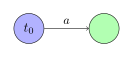
For the string :
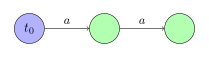
For the string :
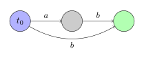
For the string :
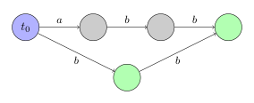
For the string :
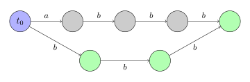
In the last example, if we directly build the AC automaton for all its suffixes, the paths and should lead to different nodes. However, both nodes are terminal states, and appending any further character will never produce a longer matching string. This shows that the two nodes have the same behavior with respect to transitions in the automaton, so they can be merged into one node. This gives the SAM shown in the figure. The discussion below extends this idea of merging nodes to all cases and explains that, as long as nodes are merged appropriately, the resulting SAM has only nodes and transitions.
A linear-complexity construction algorithm
Before describing the algorithm for constructing a SAM in linear time, we need to introduce two concepts that are important for understanding the construction and give brief proofs of their properties. The ending-position set defines the nodes in a SAM (that is, it gives the necessary and sufficient condition for nodes to be merged), while the suffix link is simply the natural counterpart of the failure pointer in an AC automaton.
Ending positions endpos
For string , consider any nonempty substring denoted . We denote by the set of all ending positions of in (assuming that the characters in the string are numbered starting from zero). For example, for the string , we have .
Two substrings and may have exactly the same ending positions: . This defines an equivalence relation among the substrings of . All nonempty substrings of can be divided into several equivalence classes according to their ending-position sets .
It is a fact that each such equivalence class corresponds to one state of the SAM1. In other words, whenever two substrings have the same ending positions, their paths in the SAM correspond to the same state. Equivalently, every non-initial state in a SAM corresponds to one or more nonempty substrings with the same . In short, the states of a SAM are the equivalence classes of all nonempty substrings, together with the initial state.
For now, accept this fact; we will use it to introduce the SAM construction algorithm. We will also show that the SAM satisfies all the required properties except minimality, which follows from the Myhill–Nerode theorem.
The values of give us several important conclusions that explain the relationship between different substrings corresponding to the same state.
Lemma 1
For string , let and be two nonempty substrings (assume ). They have the same if and only if every occurrence of in occurs as a suffix of .
Proof
The lemma is obvious. If and have the same , then is a suffix of , and in it occurs only as a suffix of . Conversely, by definition, if is a suffix of and occurs in only as a suffix of , then the two substrings have the same .
Lemma 2
Consider two nonempty substrings and (assume ). Then either or , depending on whether is a suffix of :
Proof
If the sets and have at least one common element, then since and end at the same position, is a suffix of . Therefore, wherever occurs, the substring also occurs. Hence .
Lemma 3
Consider an equivalence class of substrings with the same , and sort all substrings in the class by nonincreasing length. Then each substring is no longer than the preceding one, and it is also a suffix of the preceding one. In other words, for any two substrings in the same equivalence class, the shorter one is a suffix of the longer one, and the lengths of the substrings in the class are consecutive, taking every integer value in some interval.
Proof
If the equivalence class contains only one substring, the lemma is obvious. We now consider an equivalence class containing more than substring.
By Lemma 1, among any two distinct strings with the same , one must be longer and one shorter, and the shorter one is always a proper suffix of the longer one. Thus, no two strings in the equivalence class have the same length.
Let be the longest string in the equivalence class and the shortest. By Lemma 1, is a proper suffix of . Now consider any suffix of whose length lies in the interval . It is easy to see that this suffix is also in the same equivalence class, because it can occur in only as a suffix of (this is because the shorter suffix occurs in only as a suffix of ). Therefore, by Lemma 1, this suffix has the same as .
In one sentence, the substrings corresponding to the same state have distinct lengths, and those lengths are consecutive natural numbers; the shorter substrings are always suffixes of the longer ones.
Suffix link link
Consider a state in the SAM. We already know that state corresponds to an equivalence class of substrings with the same . Let be the longest of these strings; then all the other strings are suffixes of .
We also know that the first few suffixes of (considered in decreasing order of length) all belong to this equivalence class, while the other suffixes (at least one—the empty suffix) belong to other equivalence classes. Let be the longest among these other suffixes, and connect the suffix link of to .
In other words, for , the state reached by its suffix link corresponds to the longest suffix of whose set differs from it. It is also the longest suffix of that occurs more often in than .
For convenience, we define the equivalence class corresponding to the initial state to contain only the empty string, with .
Lemma 4
All suffix links form a tree rooted at .
Proof
Consider any state . The state reached by corresponds to a strictly shorter string (by the definition of a suffix link and Lemma 3). Therefore, by following suffix links, we always eventually reach the initial state , which corresponds to the empty string.
Lemma 5
The tree constructed with sets as nodes and set inclusion as edges (that is, the set of each child is contained in the set of its parent) is the same as the tree constructed using suffix links .
Proof
By Lemma 2, the sets of any SAM form a tree (because any two sets are either disjoint or one is a subset of the other).
Now consider any state and its suffix link . From the suffix link and Lemma 2, we obtain
Note that this should be rather than , because if , then and should be merged into one node.
Combining the preceding lemmas, we see that the tree formed by suffix links is essentially the tree formed by the sets.
Here is an example of the suffix-link tree produced when constructing a SAM for the string . Each node is labeled with the longest substring in its corresponding equivalence class.
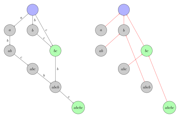
The following observations about the figure are helpful for understanding the construction algorithm and applications below.
Explanation of the figure
-
The SAM contains a longest path whose label is exactly the string itself. Starting from the initial state, each state along this path corresponds to a prefix of (). These states are crucial in the later applications.
-
The suffix-link tree can be viewed as the result of "compressing" the paths that move these "prefix states" along suffix links to the root (the initial state).
- Along each path, the sets of strings corresponding to the nodes form a partition of all suffixes of the corresponding prefix. For example, the path obtained by following suffix links from the state labeled to the root is . The node actually corresponds to the set , the node actually corresponds to , and the node corresponds to the empty string.
- Different paths may share the same node, which is why there is "compression". For example, the paths and share the node . This is because , while at position the string is immediately preceded by , and at position the string is immediately preceded by . Thus, when a character is added to the front (that is, when moving against the suffix links), the set of ending positions (and hence the state) splits.
- The suffix-link tree only needs to merge these suffix paths together appropriately; there is no need to consider other nodes. This is because every substring is a suffix of some prefix, so it must appear on one of these paths. The construction algorithm described later essentially adds characters one by one, constructs such a suffix path for each newly added prefix, and "compresses" it appropriately into the paths that already exist (that is, it does not reconstruct states or transitions that already exist).
- The terminal states are exactly all nodes on the suffix path containing the string itself.
-
Transitions reaching the same state must have the same label, and their source states must lie on some (continuous) path in the suffix-link tree. For example, there are two states with a transition to state : and . They lie on the suffix-tree path . Note that they correspond to the string sets and , respectively. Appending the character to these strings gives state , whose corresponding string set is .
- After adding a character, different states may transition to the same state because the new character makes it harder for ending positions to be added.
-
In the suffix-link tree, the set of each node is the union of the sets of its children, with at most one additional position. Moreover, this new position exists if and only if the node corresponds exactly to a prefix of the original string ending at that position. In the figure, none of the non-root, non-leaf nodes in the suffix-link tree corresponds to a prefix of , so this situation does not occur.
The suffix automaton stores information about all substrings of a string. This can be understood from two perspectives:
- The SAM itself can be viewed as a compressed version of the AC automaton for all suffixes of the string. Therefore, it stores information about all prefixes of all suffixes, which is equivalent to storing information about all substrings of the string.
- The suffix-link tree of a SAM can be viewed as a compressed version of the suffix paths of all prefixes of the string. Therefore, it stores information about all suffixes of all prefixes, which is also equivalent to storing information about all substrings of the string.
Both perspectives are useful when handling different problems.
Summary
Before discussing the algorithm itself further, let us summarize the preceding material and introduce some auxiliary notation.
-
The substrings of can be divided into equivalence classes according to their ending-position sets ;
-
A SAM consists of the initial state and one state corresponding to each equivalence class of nonempty substrings;
-
Each state matches one or more substrings. Let be the longest of them and let be its length. Similarly, let be the shortest substring and let its length be . Then all strings corresponding to this state are distinct suffixes of , and their lengths take every integer value in the interval .
-
For any state , define its suffix link as an edge to the suffix of whose length is . The suffix links starting at the root form a tree. This tree also represents the inclusion relationships between the sets.
-
For any state , can be expressed using its suffix link :
-
If we start at any state and traverse suffix links, we will always reach the initial state . In this process we obtain a sequence of pairwise disjoint intervals , whose union forms the continuous interval .
Algorithm
We can now discuss the SAM construction algorithm. This is an online algorithm: we can add the characters of the string one by one and maintain the SAM accordingly at each step.
Before discussing the detailed implementation, let us first use the figures to get an initial feeling for how the SAM may change when a new character is added.
An intuitive view of the incremental construction
Given the SAM of a string , we can construct the SAM of . According to the explanation of the figures above, we only need to construct the suffix path of the newly added prefix (namely ) and compress it into the existing paths. Furthermore, as described above, every node on the new suffix path must be reachable by a transition labeled from a node on a suffix path of the original string .
Before adding the new character to the original string , we first consider what form its suffix path can have and how it can transition through . The most general case is shown below:
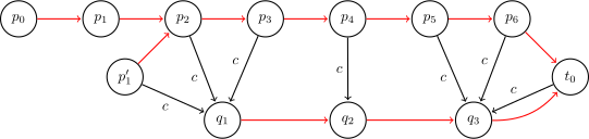
In the figure, the suffix path of the original string is , and suffix links are shown by red arrows. Some nodes (namely ) already have transitions labeled ; because appending the same character to a sequence of consecutive suffixes again produces consecutive suffixes, the endpoints of these transitions form another suffix path . There are two observations:
-
On the suffix path of the original string , the nodes without a transition labeled must be the first few nodes. Once some node (the node in the figure) has a transition labeled , every subsequent node must also have a transition labeled .
Explanation: Let . Every subsequent node corresponds to a suffix of . Thus, if also occurs in , then every suffix of followed by must also produce a substring of , so all these nodes have transitions labeled .
-
Although the nodes that can reach a node via a transition labeled must form a contiguous segment of the suffix-link tree, this segment need not lie entirely on the suffix path from to the root. In particular, only some of the initial nodes in the segment corresponding to may not be on this suffix path. For example, the node in the figure corresponds to , where is not on the suffix path of .
Explanation: Let . Then corresponds to , but clearly in the figure, because the latter is . This shows that the strings corresponding to the part of cannot be obtained by taking and its suffixes and applying transitions. Conversely, the strings in must be suffixes of , so after removing the final they must be suffixes of . In other words, the nodes with transitions labeled to must lie on the suffix path beginning at . This is why only some nodes in the initial segment corresponding to may not lie on the suffix path of .
What changes when we add a character to the end of the original string —that is, add —and construct the corresponding suffix path? The answer is shown below:
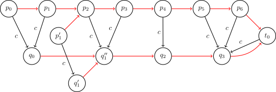
Since node is reached from the node corresponding to the original string by a transition labeled , it corresponds to the new string . Thus, its suffix path is the newly added suffix path. If a node on the old suffix path already has a transition labeled , the new suffix path must also pass through the node reached by that transition, so we can directly reuse the old node. The new suffix path contains exactly one completely new node, , which receives the transitions from the initial nodes on the old suffix path that did not have transitions labeled .
Besides these obvious facts, note that the old node is also copied once, or equivalently split into two nodes . This is because the newly added suffix path overlaps the existing paths only partially: among the strings corresponding to the old node , only the shorter ones (those reachable from nodes and ) appear on the new suffix path, while the longer ones (those reachable from node ) do not. Therefore the new suffix path can pass through only part of node , which must be split into two nodes to represent this situation. For the same reason, as explained above, the nodes and after cannot be reached by transitions from nodes not on the suffix path of , so all strings corresponding to these nodes appear on the new suffix path and no split is needed.
In terms of what states represent in a SAM, each state is an set. Suppose the new ending position when the string is extended is . Then the new node has ending-position set , while the split nodes and correspond to the sets and , respectively. The later nodes and in fact also gain in their existing ending-position sets. In other words, although , , and their associated transitions do not change, the sets they represent do become larger.
The above describes the most complex and general case (namely case 3 below). In practice, node may not exist, so no split is needed (namely case 2 below). To determine this case, it is enough to check whether , equivalently . It is also possible that none of the nodes on the suffix path of has a transition labeled ; then only the new node needs to be created (namely case 1 below).
Now that we understand the idea of the new suffix path, let us discuss the concrete steps of incremental construction.
Process
To keep the space complexity linear, we store only the values of and and the transition list of each state. We do not mark terminal states (but we will show later how to assign these marks after constructing the SAM).
Initially, the SAM contains only one state , numbered (the other states are numbered ). For convenience, for state , set and ( denotes a virtual state).
We only need to implement the process of adding a character to the current string. The algorithm is as follows:
SAM incremental construction process
-
Let be the state corresponding to the entire string before character is added (initially, set ; the final step of the algorithm updates ).
-
Create a new state and set to ; at this point the value of is unknown.
-
Now perform the following process: starting from state , if the current state does not yet have a transition labeled , add a transition labeled to state and move the current state along its suffix link. If we encounter a state that already has a transition labeled , stop and mark this state as .
-
Case 1: If no such state is found, we have reached the virtual state ; set to and exit.
-
Suppose now that we have found a state with a transition labeled . Mark the state reached by this transition as . Then either or .
-
Case 2: If , simply set to and exit.
-
Case 3: Otherwise, the situation is more complicated and we need to clone state : create a new state , copying all information from except its value (including its suffix link and transitions). Set to .
After cloning, set the suffix link from to , and also set the suffix link from to .
Finally, walk back along suffix links from state . Whenever a visited state has a transition to state , reconnect that transition to state .
-
After handling all three cases above, update to state .
If we also want to know which states are terminal states and which are not, we can find all terminal states after constructing the complete SAM for . To do so, start from the state corresponding to the entire string (stored in the variable ) and traverse its suffix links until reaching the initial state. Mark every state visited as a terminal state. It is easy to see that this marks exactly all suffixes of , and these states are terminal states.
Because we create only one or two new states for each character of , the SAM has only a linear number of states. The facts that the SAM also has a linear number of transitions and that the algorithm runs in linear total time will be explained later.
Explanation
We now explain the details of each step of the algorithm and establish its correctness.
Detailed explanation of the algorithm
-
If a transition satisfies , we call it a continuous transition. Otherwise, when , it is called a non-continuous transition.
As can be seen from the algorithm description, continuous and non-continuous transitions are handled differently. Continuous transitions are fixed; we never change them again. In contrast, when a new character is inserted into the string, a non-continuous transition may change (the endpoint of the transition edge may change).
-
To avoid ambiguity, before the current character is inserted into the SAM, denote the string by .
-
The algorithm starts by creating a new state corresponding to the entire string . The reason for creating a new node is clear. At the same time, we also create a new character and a new equivalence class.
-
After creating a new state, we move from the state corresponding to the entire string , namely , along suffix links. For every state visited, we try to add a transition labeled to the new state .
However, we can add only transitions that do not conflict with existing transitions. Therefore, as soon as we find an existing transition labeled , we must stop.
-
The simplest case is that we reach the virtual state , which means that every suffix of has received a transition labeled . This also means that character has never appeared in . Therefore, the suffix link of is state .
-
In the second case, we find an existing transition . This means that we are trying to add to the automaton a string that already exists (where is a suffix of , and the string has already appeared as a substring of ). Since we assume that the construction of the automaton for is correct, we should not add a new transition here.
The difficulty, however, is determining which state the suffix link from should point to. We need to link it to a state whose longest corresponding string is exactly , so that the state's should be . Such a state may not exist, namely when . In that case, we must split state to create such a state.
-
Of course, if transition is continuous, then . In this case everything is simple: we only need to make the suffix link of point to state .
-
Otherwise, the transition is non-continuous, namely . This means that state corresponds not only to the suffix of length , but also to longer substrings of . We have no choice but to split state into two substates, so the length of the first substate is .
How do we split a state? We clone state , producing a state , and set to . Since we do not want to change paths passing through , we copy all transitions of to . We also set the suffix link from to the target of 's suffix link, and set the suffix link of to .
After splitting the state, set the suffix link from to .
In the final step, we reconnect some transitions that originally pointed to to . Which transitions need to be modified? It is enough to reconnect exactly the suffixes of all strings , where is the longest string corresponding to state . In other words, we continue moving along suffix links from node until reaching the virtual state , or until the current state's transition labeled no longer points to state .
Linear time complexity
Assume that the alphabet size is a constant, so that searching for a transition, adding a transition, and finding the next transition for one character all take time. If the transitions of each node are stored both in an array of length (for quickly looking up the transition with a given label) and in a dynamic list (for quickly traversing all available transitions), trading space for time, then the time complexity2 of the algorithm is and its space complexity is .
Proof
If we consider the different parts of the algorithm, there are three places whose time complexity is not obviously linear:
- The first is traversing all suffix links of and adding transitions labeled .
- The second is copying transitions when state is copied to a new state .
- The third is modifying transitions pointing to and reconnecting them to .
We use the fact that the size of a SAM (the number of states and transitions) is linear (the proof that the number of states is linear is the algorithm itself; the proof that the number of transitions is linear is given after the implementation).
Therefore, the total complexity of the first and second parts above is clearly linear, because each operation adds only one new transition to the automaton in amortized terms.
We still need to estimate the total complexity of the third part, in which transitions initially pointing to are reconnected to . Let , which is a suffix of . On each iteration, the length of decreases, so the starting position of as a suffix of necessarily moves to the right. Therefore, the number of times that moves along suffix links in the loop is no more than the distance by which the starting position of as a suffix of moves to the right. Since must move at least once to terminate the loop, and since is at least the result of moving once along a suffix link, when the loop terminates the starting position of as a suffix of is no earlier than that of . Moreover, when the loop terminates, the starting position of as a suffix of is exactly the starting position of as a suffix of ; as a suffix of , the string is exactly . Since is the updated value of , the number of moves in the loop is no more than the distance by which moves to the right as a suffix of the current string between its old and new values, plus one (the move needed to terminate the loop).
Because the position of the string as a suffix of the current string increases monotonically throughout the entire SAM construction3, its total movement is at most . This shows that the number of iterations in the loop modifying transitions pointing to is at most . This is exactly what we needed to prove.
Of course, if the alphabet size is not constant, the time complexity of a SAM is not linear. The transitions leaving a node must be stored in a balanced tree supporting fast lookup and insertion. Thus, if is the alphabet and is its size, the asymptotic time complexity of the algorithm is and the space complexity is .
Implementation
First, we implement a data structure that stores all information about a transition. If necessary, you can add a terminal marker or some other information here. We store the transition list in a map, allowing us to process the whole string in total space and time. Of course, when the alphabet size is a small constant (for example, 26), it is more convenient to declare next as int[K].
struct state {
  int len, link;
  std::map<char, int> next;
};
The SAM itself will be stored in an array of state structures. We record the current automaton size sz and the variable last, the state corresponding to the entire current string.
constexpr int MAXLEN = 100000;
state st[MAXLEN * 2];
int sz, last;
We define a function to initialize the SAM (creating a SAM containing only the initial state).
void sam_init() {
  st[0].len = 0;
  st[0].link = -1;
  sz++;
  last = 0;
}
Finally, we give the implementation of the main function: add a character to the end of the current string and build the automaton accordingly on top of the previous one.
Implementation
void sam_extend(char c) {
  int cur = sz++;
  st[cur].len = st[last].len + 1;
  int p = last;
  while (p != -1 && !st[p].next.count(c)) {
    st[p].next[c] = cur;
    p = st[p].link;
  }
  if (p == -1) {
    st[cur].link = 0;
  } else {
    int q = st[p].next[c];
    if (st[p].len + 1 == st[q].len) {
      st[cur].link = q;
    } else {
      int clone = sz++;
      st[clone].len = st[p].len + 1;
      st[clone].next = st[q].next;
      st[clone].link = st[q].link;
      while (p != -1 && st[p].next[c] == q) {
        st[p].next[c] = clone;
        p = st[p].link;
      }
      st[q].link = st[cur].link = clone;
    }
  }
  last = cur;
}
As mentioned earlier, if you trade memory for time (space complexity , where is the alphabet size), you can construct a SAM for an alphabet of arbitrary size in time2. However, you need to store for each state an array of size (for quickly finding the corresponding transition by character) and a list containing all available transitions (for quickly traversing all available transitions).
More properties
Number of states
For a string of length , denoted , the number of states in its SAM does not exceed (assuming ).
Proof
The algorithm itself proves this claim. At the beginning the automaton contains one state; the first and second iterations create only one node each, and each of the remaining steps creates at most states.
We can also prove this bound without using the algorithm. Recall that the number of states equals the number of distinct sets. These sets form a tree (the set of a parent contains the set of a child). Consider slightly modifying this tree: whenever it has an internal node with only one child (which means that the child's set omits at least one position from the parent's set), create a child whose set contains those omitted positions. In the end, we obtain a tree in which every internal node has degree greater than one, and the number of leaves is at most . Such a tree has at most nodes, so the number of distinct sets in the original tree is also at most .
The string reaches this upper bound: from the third iteration onward, every iteration splits a state, ultimately producing exactly states.
Number of transitions
For a string of length , denoted , the number of transitions in its SAM does not exceed (assuming ).
Proof
We first estimate the number of continuous transitions. Consider the spanning tree formed by the longest paths from state to all states in the automaton. The spanning tree contains only continuous edges, so its number of edges is less than the number of states, and hence no more than .
We now estimate the number of non-continuous transitions. Let the current non-continuous transition be , with character . Consider its corresponding string , where corresponds to a longest path from the initial state to , and corresponds to a longest path from to any terminal state. On the one hand, the strings of the form corresponding to different non-continuous transitions are distinct (because and consist only of continuous transitions). On the other hand, by the definition of terminal states, every string of the form is a suffix of the whole string . Since has nonempty suffixes, and none of the strings of the form is itself (because the whole string consists only of continuous transitions), the total number of non-continuous transitions is at most .
Adding the two estimates above gives the upper bound . However, the maximum number of states can occur only in cases like , and in that case the number of transitions is clearly less than .
Therefore we obtain the tighter upper bound for the number of SAM transitions. The string reaches this bound.
Suffix-link tree
Although SAM construction is intended to obtain information about its states and transitions, the suffix links recorded during construction and the corresponding longest-substring lengths are often more important in applications than the SAM transitions, and can even be used independently of the transitions.
During SAM construction, the value of the state must be updated. It corresponds to the string before (and after) each character is added, that is, every prefix of . Let the state corresponding to the -th prefix be ; then we obtain the states , totaling states. In addition, define the initial state as , corresponding to the empty prefix. We will refer to these states as "prefix nodes" for now.
As mentioned in Lemma 4, all states and suffix links form a rooted tree with root . This tree is also called the suffix-link tree (Chinese OI contestants often call it the parent tree). It records all suffixes of all prefixes of the string, that is, all substrings.
The suffix-link tree has the following properties:
- The string corresponding to an ancestor node is always a suffix of the string corresponding to a descendant node.
- The set at each node is exactly the set of all indices of "prefix nodes" in its subtree.
- The set of an ancestor in the suffix-link tree always strictly contains the set of a descendant.
- The value at each node is the length of the longest common suffix of all prefixes corresponding to the "prefix nodes" in its subtree.
- Except for the root , the number of distinct substrings corresponding to each node is its value minus the value of its parent, namely .
These properties have many applications. For example, the longest common suffix of the -th and -th prefixes is the string corresponding to the longest string of the LCA of and .
Finally, the suffix-link tree built for a string has the same structure as the suffix tree built for its reverse . This is often used to construct a suffix tree offline.
Applications
Let us look at some problems that can be solved using a SAM. For simplicity, assume that the alphabet size is a constant. This allows us to treat the complexity of adding and traversing a character as constant.
Checking whether a string occurs
Problem
Given a text string and several pattern strings , determine whether occurs as a substring of .
Solution
In time , we construct a suffix automaton for the text string . To check whether a pattern string occurs in , we start at and follow transitions according to the characters of . If at some point no transition is available, then is not a substring of . If we process the entire string this way, then the pattern occurs in .
For each string , the time complexity of the algorithm is . In addition, this algorithm finds the maximum prefix length of that occurs in the text string.
Number of distinct substrings
Problem
Given a string , count the number of distinct substrings.
Solution 1
Construct a suffix automaton for the string .
Every substring of corresponds to some path in the automaton. Therefore, the number of distinct substrings equals the number of distinct paths starting at in the automaton.
Since the SAM is a directed acyclic graph, the number of paths can be computed by dynamic programming. Let be the number of paths starting from state (including the path of length zero). Then we have the recurrence:
That is, is the sum over the endpoints of all transitions from ; the triple in means that the suffix automaton has a transition from to via .
Thus, the number of distinct substrings is (because the empty substring must be removed).
The total time complexity is .
Solution 2
Another method is to use the information in the suffix-link tree after constructing the suffix automaton. The number of substrings corresponding to each node is ; summing this over all automaton nodes gives the answer.
The total time complexity is still .
Example problems: 【Suffix Automaton (Template)】, SDOI2016 Generating Magic
Total length of all distinct substrings
Problem
Given a string , calculate the total length of all distinct substrings.
Solution 1
The solution to this problem is similar to that of the previous problem, except that we now need to perform dynamic programming in two parts: the number of distinct substrings and their total length .
We introduced how to calculate in the previous problem. The value of can be calculated by the following recurrence:
We take the answer for each adjacent node and add , because every substring starting from state gains one character.
The time complexity of the algorithm is still .
Solution 2
We can likewise use information from the suffix-link tree. The total lengths of all suffixes of the longest substring corresponding to each node are
and subtracting the corresponding value for its node gives the net contribution of that node. Summing over all nodes of the automaton is sufficient.
The total time complexity is still .
The k-th Largest Substring in Lexicographic Order
Problem
Given a string and multiple queries. For each query, given , find the largest substring of that is the -th in lexicographic order.
Solution
The idea for solving this problem can be developed from the ideas used for the first two problems. The -th largest substring in lexicographic order corresponds to the -th largest path in the SAM. Therefore, after calculating the number of paths from each state, we can easily find the -th largest path starting from the root of the SAM.
The preprocessing time complexity is , and the complexity of a single query is , where is the query answer and is the size of the character set.
Note
Although this is a classic suffix-automaton problem, suffix arrays are actually the most convenient choice because the problem involves lexicographic order.
Example problems: SPOJ - SUBLEX, TJOI2015 String Theory
Minimum Cyclic Shift
Problem
Given a string , find its lexicographically smallest cyclic shift.
Solution
It is easy to see that contains all cyclic shifts of as substrings.
Thus the problem reduces to finding, in the suffix automaton of , the smallest path of length . This can be done trivially: starting from the initial state, greedily follow the smallest character.
The total time complexity is .
Occurrence Count
Problem
Given a text string and multiple queries, each providing a pattern string , determine how many times the pattern string occurs as a substring in .
Solution 1
Using information from the suffix-link tree, we can preprocess the size of the set of every node with a DFS.
Initialize the set size of every “prefix node” to , and that of every non-“prefix node” to . Then, while traversing upward along suffix links from the bottom, add the set sizes of all child nodes to each parent node (do not omit the parent's own initial value). The resulting value at each node is the size of its set. The reason the set sizes of different child nodes can be added directly is that the same appears in only one subtree, so the addition does not duplicate anything.
During a query, find the node corresponding to the pattern string in the automaton. If it exists, the answer is the size of that node's set; otherwise, the answer is .
The preprocessing time complexity is , and the time complexity of a single query is .
Solution 2
Construct a suffix automaton for the text string .
Then preprocess, for every state in the automaton, a value equal to the size of the set. In fact, all substrings corresponding to the same state occur the same number of times in the text string ; this is the number of positions in the set.
However, we cannot explicitly construct the sets, so we only consider their sizes .
To calculate these values, perform the following operations. For each state, if it was not created by copying (and is not the initial state ), initialize its to 1. Then traverse all states in decreasing order of their length and add the current value of to the state pointed to by its suffix link:
After this, the answer for every state is correct.
Why is this correct? There are exactly states that were not obtained by copying, and the first of them were created when the first characters were inserted. Thus, for each such state, when it is processed, we count the number of positions corresponding to it. We therefore initially set the of these states to and the of all other states to .
Next, for each , perform the following operation: . Its meaning is that if a string occurs times, all of its suffixes end at exactly the same positions, and therefore also occur times.
Why do we not count any position more than once in this process? Because we add the positions of one state to only one other state, so a state cannot point its positions to another state in two different ways.
Therefore, in time, all state values can be calculated.
Finally, answering a query only requires looking up , where is the state corresponding to the pattern string. If the pattern string does not exist, the answer is . The time complexity of a single query is .
First Occurrence Position
Problem
Given a text string and multiple queries, return the position of the first occurrence of the string in , that is, the starting position of .
Solution 1
Using information from the suffix-link tree, we can preprocess the minimum value in the set of every node with a DFS.
Initialize every “prefix node” to , and every non-“prefix node” to . Then, while traversing upward along suffix links from the bottom, compare each parent's value with the values of all its child nodes and take the minimum (do not omit the parent's own initial value). The resulting value at each node is the minimum value in its set.
During a query, find the node corresponding to the pattern string in the automaton. If it exists, the answer is its value minus ; otherwise, the answer does not exist.
The preprocessing time complexity is , and the time complexity of a single query is .
Solution 2
Construct a suffix automaton. For every state in the SAM, preprocess the position . That is, for each state , find the position where a string represented by this state first occurs, . In other words, find the minimum element of each set (although we obviously cannot maintain all sets explicitly).
To maintain these positions, extend the function sam_extend(). When creating a new state , set
When copying node to , set
(The only other possible value, , is clearly too large.)
The answer to a query is then , where is the state corresponding to the string . A single query takes only time.
All Occurrence Positions
Problem
The problem is the same as above; this time, given the text string , find all positions where the pattern string occurs.
Solution 1
After finding the node corresponding to the pattern string , traverse its subtree using information from the suffix-link tree, and output a position whenever a terminal node is found.
The complexity of a single query is , where is the answer to the query. As in the proof that the number of states is linear, the size of a subtree in the suffix-link tree is no more than twice the size of that node's set, so the subtree traversal has complexity .
Solution 2
Again, construct a suffix automaton for the text string . As in the previous problem, calculate for every state.
If is the state corresponding to the pattern string , then is clearly one of the answers. We have already found the state corresponding to in the automaton. Which other positions do we need to find? They are precisely those corresponding to strings that have as a suffix. In other words, we need to find all states from which state can be reached by suffix links.
Therefore, to solve this problem, we need to store, for each state, a list of suffix links pointing to it. The query answer consists, for every state found by performing DFS or BFS from state using only reversed suffix links, of its value.
The preprocessing complexity is , and the complexity of a single query is .
We never visit a state more than once, because each state has only one suffix link, so there cannot be two different paths to the same state.
We only need to consider different states that may have the same value. This happens only when one state is copied from another. However, this does not affect the complexity analysis. As in the proof that the number of states is linear, the number of such states whose suffix is is no more than .
Moreover, we can remove duplicate positions by ignoring the values of copied nodes. In fact, for a state, if it can be reached through the copied state, it can also be reached through the original state. Thus, if we record a marker is_clone for each state to indicate whether it was copied, we can simply ignore copied states and output the values of all other states.
The following is a rough implementation:
struct state {
  bool is_clone;
  int first_pos;
  std::vector<int> inv_link;
  // some other variables
};

// After constructing the SAM
for (int v = 1; v < sz; v++) st[st[v].link].inv_link.push_back(v);

// Output all occurrence positions
void output_all_occurrences(int v, int P_length) {
  if (!st[v].is_clone) cout << st[v].first_pos - P_length + 1 << endl;
  for (int u : st[v].inv_link) output_all_occurrences(u, P_length);
}
Shortest String That Does Not Occur
Problem
Given a string and a particular character set, find the shortest string that does not occur in .
Solution
Perform dynamic programming on the suffix automaton of string .
Suppose that we have already processed part of the substring and are currently at state . Let the minimum number of characters that must be added at state to obtain a transition that does not occur be .
Computing is simple. If there is no transition using at least one character from the character set, then . Otherwise, adding one character is not enough, and we take the minimum over all transitions:
The answer is , and the string can be reconstructed backward using the computed array .
Longest Common Substring of Two Strings
Problem
Given two strings and , find the longest string that occurs as a substring in both and ; call this string .
Solution
Construct a suffix automaton for string .
We now process string . For every prefix, find the longest suffix of that prefix that occurs in . In other words, for every position in , find the length of the longest common substring of and ending at that position.
To do this, use two variables, current state and current length . They describe the currently matched part: its length and the state corresponding to it.
Initially, and , meaning that the match is the empty string.
We now describe how to add a character and recompute the answer:
-
If there is a transition from using character , simply follow it and increment .
-
If no such transition exists, shorten the current match, which means following a suffix link:
At the same time, shorten the current length. We clearly need to set to , because the longest string corresponding to the state reached through this suffix link is a substring.
-
If there is still no transition using this character, continue following suffix links and decreasing until a transition is found or the virtual state is reached. The latter means that character does not occur in at all, so set .
Clearly, the answer is the maximum of all values of .
The time complexity of this part is , because each move either increases by one or moves along suffix links several times, decreasing on each move.
Code:
string lcs(const string &S, const string &T) {
  sam_init();
  for (int i = 0; i < S.size(); i++) sam_extend(S[i]);

  int v = 0, l = 0, best = 0, bestpos = 0;
  for (int i = 0; i < T.size(); i++) {
    while (v && !st[v].next.count(T[i])) {
      v = st[v].link;
      l = st[v].length;
    }
    if (st[v].next.count(T[i])) {
      v = st[v].next[T[i]];
      l++;
    }
    if (l > best) {
      best = l;
      bestpos = i;
    }
  }
  return T.substr(bestpos - best + 1, best);
}
Example problem: SPOJ Longest Common Substring
Longest Common Substring of Multiple Strings
Problem
Given strings , find their longest common substring, that is, a string that occurs as a substring in every string.
Solution 1
Concatenate all the substrings into one longer string , separating each string with a special character (one character for each string):
Then construct a suffix automaton for string .
We now need to find, in the automaton, a string that occurs in every string . The added special characters are useful here. If contains a substring , then from the node corresponding to substring , denoted , there must be a path to that passes through none of the other special characters . For a common substring , such a path must exist for every special character .
Thus we need to calculate reachability: for every character and every state in the automaton, determine whether such a path exists. This can be computed easily with DFS or BFS and dynamic programming. The answer is the longest among the states that can reach all special characters.
Solution 2
Without loss of generality, let be the shortest string and construct a SAM for it. Use the algorithm for the longest common substring of two strings to calculate the longest common substring length between each remaining string and . During matching, each time a character from a string is matched, we move accordingly in the SAM, so we can directly record the length of the longest substring of that each SAM state can match during the matching process.
During matching, whenever a SAM state is reached, all its ancestors in the suffix-link tree are necessarily matched at the same time, but the matching-length information for the ancestors is not updated. Therefore, after matching string , update along suffix links from bottom to top, propagating the longest matched-substring information from child nodes to parent nodes. Be careful that the longest matching length recorded at a parent cannot exceed its own value. This yields the length of the longest substring that each state in the SAM of can actually match in .
Finally, match every once, take the minimum over the actually matched lengths recorded at each SAM state, and obtain the length of the longest common substring of that each state can actually match. Then traverse all SAM states and take the maximum; this is the length of the longest common substring of the strings.
The time complexity is . Although the SAM of is traversed times, is the smallest, so ; the dominant term in the complexity is still the matching process that traverses all substrings.
Example problem: SPOJ Longest Common Substring II
Exercises
- P3804 Template Suffix Automaton
- SDOI2016 Generating Spells
- SPOJ - SUBLEX
- TJOI2015 String Theory
- SPOJ Longest Common Substring
- SPOJ Longest Common Substring II
- Codeforces 1037H Security
- Codeforces 666E Forensic Examination
- HDU4416 Good Article Good sentence
- HDU4436 str2int
- HDU6583 Typewriter
- Codeforces 235C Cyclical Quest
- CTSC2012 Familiar Article
- NOI2018 Your Name
Related Resources
Here are some of the earliest works related to SAM:
- A. Blumer, J. Blumer, A. Ehrenfeucht, D. Haussler, R. McConnell. Linear Size Finite Automata for the Set of All Subwords of a Word. An Outline of Results. [1983]
- A. Blumer, J. Blumer, A. Ehrenfeucht, D. Haussler. The Smallest Automaton Recognizing the Subwords of a Text. [1984]
- Maxime Crochemore. Optimal Factor Transducers. [1985]
- Maxime Crochemore. Transducers and Repetitions. [1986]
- A. Nerode. Linear automaton transformations. [1958]
This topic can also be found in newer resources and in many books on string algorithms:
- Maxime Crochemore, Rytter Wowjcieh. Jewels of Stringology. [2002]
- Bill Smyth. Computing Patterns in Strings. [2003]
- Bill Smith. Methods and algorithms of calculations on lines. [2006]
Additional resources:
- Suffix Automaton, Chen Lijie.
- Extensions of Suffix Automata on Trie Trees, Liu Yanyi.
- Suffix Automata and Their Applications, Zhang Tianyang.
- https://www.cnblogs.com/zinthos/p/3899679.html
- https://codeforces.com/blog/entry/20861
- https://zhuanlan.zhihu.com/p/25948077
This page was mainly translated from the article Суффиксный автомат and its English translation Suffix Automaton. The Russian version is licensed under Public Domain + Leave a Link; the English version is licensed under CC-BY-SA 4.0.
Footnotes
-
The reason for taking every state to be an equivalence class is essentially the Myhill–Nerode theorem mentioned in this section. In simple terms, if two strings and have different sets, they cannot correspond to the same state of the SAM: the paths from the same state to terminal states are always the same, which means that the ways of appending characters to the ends of and to reach the end of are also the same; this is precisely what says that and end at the same positions in . Conversely, as long as two strings and have the same set, they can correspond to the same state of the SAM. The proof that this is possible is the content of Nerode's theorem and is not discussed here. Nevertheless, the discussion at least makes it plausible that placing strings with the same set in one state produces a minimal SAM, because further merging of nodes is impossible. ↩
-
If we do not additionally use a list to record the available transitions of the current state, but use an array storing all possible transitions (whether or not they exist) and copy it directly when copying a node, the time complexity is also . ↩ ↩2
-
What the main text does not explain here is whether the position of is also monotonically nondecreasing in the first and second cases. The first case is easy to verify, because after the update, is the empty string, whose start and end positions are at the end of string . In the second case, the transition is continuous, which means . However, adding a new character to the end of a substring only makes it harder for that substring to occur in the string. In other words, when the set of end positions of the suffix of of length strictly contains , the set of end positions of the suffix of of length may still be the same as . Hence , which means that the starting position of as a suffix of is no later than the starting position of as a suffix of . When a state for which a transition via exists is found, at least one move must have been made, which means that the starting position of as a suffix of is no earlier than the starting position of as a suffix of . Finally, . This shows that, in the second case, the position of is also monotonically increasing. ↩