AIOJ

Introduction

The Garsia–Wachs algorithm is an efficient algorithm for constructing optimal binary search trees and alphabetic Huffman codes in linear time. It is named after Adriano Garsia and Michelle L. Wachs, who published the relevant paper in 1977.

Problem Statement

Given an integer $n$ and $n+1$ nonnegative weights $w_{0},w_{1},\dots ,w_{n}$ , construct a rooted binary tree in which each of the $n$ internal nodes has two children, so the tree has $n+1$ leaves. Map the input sequence of length $n+1$ to the leaves in order. The goal is to find, among all possible trees with $n$ internal nodes, one minimizing the weighted sum of the path lengths from the root to the leaves.

Optimal Binary Search Trees

This problem can be viewed as constructing a binary search tree for $n$ ordered keys, assuming that the tree is used only to search for values absent from the tree. The $n$ keys divide the search space into $n+1$ intervals, and the weight of an interval can represent the probability that the searched value lies in it. The weighted external path length determines the expected search time.

Alphabetic Huffman Codes

The same problem can be used to construct a Huffman code. It explicitly encodes $n+1$ given values using variable-length binary strings. In this interpretation, a value's code is the sequence of left and right steps from the root to its leaf (for example, left is $0$ and right is $1$ ). Unlike a standard Huffman code, this code is alphabetic: the order of the binary codes is the same as the order of the input values. If a value's weight is its frequency in a message, the Garsia–Wachs algorithm outputs an alphabetically ordered Huffman code that minimizes the encoded message length.

Process

The Garsia–Wachs algorithm generally has three stages:

Build a binary tree whose values are at the leaves; its order may initially be wrong.
Compute the distance from the root to every leaf.
Build another binary tree with the same leaf distances but the correct order.

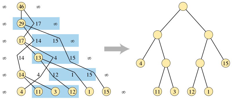
As shown above, the first stage builds a binary tree by repeatedly merging unordered triples from the input sequence (on the left), while the algorithm outputs a correctly ordered binary tree whose leaf heights are the same as those of the first tree.

The first stage is easier to describe if two sentinel values $\infty$ (or sufficiently large finite values) are added at the beginning and end of the sequence. Thus, in contest solutions using Garsia–Wachs for an array $\mathit{num}$ of length $n$ , we usually define $\mathit{num}[0] = \mathit{num}[n+1] = \infty$ .

The first stage maintains a forest initially consisting of one-node trees, one for each non-sentinel input weight. Each tree has an associated value equal to the sum of the weights of its leaves. To maintain the sequence of these values, there is one sentinel at each end. The initial sequence is simply the input order of the leaf weights. Repeat the following steps, each of which shortens the sequence, until only one tree contains all leaves:

Find three consecutive weights $x$ , $y$ , $z$ in the sequence such that $x \leq z$ . Such a triple always exists because the sentinel at the end is larger than any two preceding finite values.
Remove $x$ and $y$ from the sequence and create a new tree node as the parent of the $x$ and $y$ nodes, with value $x+y$ .
Reinsert the new node immediately after the nearest value before the original position of $x$ that is greater than or equal to $x+y$ . Such a position, measured from the original position of $x$ , always exists because of the left sentinel.

For an efficient implementation, the current sequence can be maintained in any balanced binary-search-tree structure. This allows $x$ and $y$ to be removed and their new parent to be inserted in logarithmic time. At every step, the weights at even indices up to $y$ form one decreasing sequence, and the weights at odd indices form another decreasing sequence. Therefore, the insertion position of $x+y$ can be found with two binary searches on these two decreasing sequences, each supported by a balanced tree. By linearly searching from the $z$ value of the previous triple, the first position satisfying $x \leq z$ can be found in total linear time.

The proof of the third stage—that another tree with the same distances exists and gives an optimal solution—is important. However, there are several proofs and they are too involved to include here. Assuming the third stage is correct, the second and third stages are straightforward to implement in linear time. Therefore, on an input sequence of length $n$ , the total time complexity of the Garsia–Wachs algorithm is $O(n\log n)$ .

Applications

The Haskell garsia-wachs package provides a functional implementation of the Garsia–Wachs algorithm. It is mainly used to construct optimal search trees or to balance the rope data structure optimally.

Note

rope is a Haskell tool for operating on byte strings (bytestrings), with optional annotations, using a finger tree.

Examples

POJ 1738 An old Stone Game

This is an old stone-merging game. At the beginning, the player arranges $n$ ( $1 \leq n \leq 50000$ ) piles of stones in a row. The goal is to merge them into one pile. At each step, two adjacent piles may be merged into a new pile. The score is the total number of stones in the new pile. Compute the minimum possible total score.

Solution idea

Stone merging is a classic problem that can generally be solved with interval DP. When the data is large, however, such as $n$ ( $1 \leq n \leq 50000$ ) here, the Garsia–Wachs algorithm is more efficient. First initialize an array of size $n$ , $\mathit{num}[n]$ , with $\mathit{num}[0] = \mathit{num}[n+1] = \infty$ . Then repeatedly find the smallest $i$ satisfying $\mathit{num}[i-1] \leq \mathit{num}[i+1]$ , merge $\mathit{num}[i-1], \mathit{num}[i]$ into $\mathit{temp}$ , and find the largest preceding $j$ with $\mathit{num}[j] > \mathit{temp}$ , then move $\mathit{temp}$ after $j$ . Repeat this step until $1$ pile remains. The requirement that only adjacent piles may be merged is respected: since $\mathit{num}[j]\geq \mathit{num}[i-1] + \mathit{num}[i]$ , we may regard $\mathit{num}[j+1]$ through $\mathit{num}[i-2]$ as one $\mathit{num}[mid]$ block, so $\mathit{sum}$ is necessarily merged first. Thus the rule is not violated.

ATCODER N-Slimes

$N$ slimes are arranged in a row. Initially, the $i$ -th slime from the left has size $a_{i}$ . Taro repeatedly combines two adjacent slimes into one until only one remains. If the new slime has size $x+y$ , where $x$ and $y$ are the sizes before the combination, and the operation costs $x+y$ . The relative order of the slimes does not change. Find the minimum possible total cost.

Garsia–Wachs Algorithm