AIOJ

Introduction

Simulated annealing is a randomized algorithm. When a problem has a huge (or even infinite) number of candidate solutions and is not unimodal, we often use simulated annealing to solve it.

Explanation

From the process of the hill-climbing algorithm, we can see that the hill-climbing algorithm directly discards a non-optimal solution near the current optimum. In many cases, however, we need to accept such a non-optimal solution in order to escape the local optimum; this is the simulated annealing algorithm.

What is annealing? (excerpted from Baidu Baike)

Annealing is a metal heat-treatment process in which metal is slowly heated to a certain temperature, held there for a sufficient time, and then cooled at an appropriate rate. Its purposes are to reduce hardness and improve machinability; eliminate residual stress, stabilize dimensions, and reduce the tendency toward deformation and cracking; refine grains, adjust the microstructure, and eliminate structural defects. Strictly speaking, annealing is a heat-treatment process for materials, including metallic and non-metallic materials. The purpose of annealing new materials may also share similarities and differences with that of traditional metal annealing.

Because the principles of annealing introduce more random factors, the probability of obtaining an optimal solution increases greatly. We can therefore simulate this process, taking the objective function as the energy function.

Process

In one sentence: if the new state is better, update the answer; otherwise, accept the new state with a certain probability.

Let the current temperature be $T$ , and let the energy (value) difference between the new state $S'$ and the known state $S$ (the new state is obtained randomly from the known state) be $\Delta E$ ( $\Delta E\geqslant 0$ ). Then the probability of a state transition (updating the best solution) is

P(\Delta E)= \begin{cases} 1, & S' \text{ is better than } S,\\ \mathrm{e}^\frac{-\Delta E}{T}, & \text{otherwise}. \end{cases}

Note: To obtain a higher-quality solution, we sometimes randomly generate multiple states near the solution found at the current temperature after simulated annealing ends, attempting to find a better solution (the process is similar to simulated annealing).

How to anneal (cool down)

Simulated annealing has three parameters: the initial temperature $T_0$ , the cooling factor $d$ , and the terminal temperature $T_k$ . Here $T_0$ is relatively large, $d$ is very close to $1$ but less than $1$ , and $T_k$ is a positive number close to $0$ .

First set $T=T_0$ , perform one transition attempt according to the steps above, and then set $T=d\cdot T$ . When $T<T_k$ , the simulated annealing process ends, and the current best solution is the final optimal solution.

To make the solution more accurate, we usually do not directly use the current solution as the answer; instead, we maintain the best value among all solutions encountered during annealing.

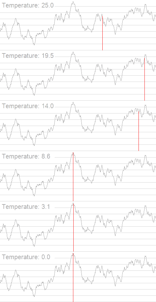
Here is an image from Simulated annealing - Wikipedia (as the temperature decreases, jumps become less random and the optimal solution becomes more stable).

Implementation

The following code uses BZOJ 3680: Beating XXX (finding the weighted geometric median of $n$ points) as an example.

#include <cmath>
#include <cstdlib>
#include <ctime>
#include <iomanip>
#include <iostream>

constexpr int N = 10005;
int n, x[N], y[N], w[N];
double ansx, ansy, dis;

double Rand() { return (double)rand() / RAND_MAX; }

double calc(double xx, double yy) {
  double res = 0;
  for (int i = 1; i <= n; ++i) {
    double dx = x[i] - xx, dy = y[i] - yy;
    res += sqrt(dx * dx + dy * dy) * w[i];
  }
  if (res < dis) dis = res, ansx = xx, ansy = yy;
  return res;
}

void simulateAnneal() {
  double t = 100000;
  double nowx = ansx, nowy = ansy;
  while (t > 0.001) {
    double nxtx = nowx + t * (Rand() * 2 - 1);
    double nxty = nowy + t * (Rand() * 2 - 1);
    double delta = calc(nxtx, nxty) - calc(nowx, nowy);
    if (exp(-delta / t) > Rand()) nowx = nxtx, nowy = nxty;
    t *= 0.97;
  }
  for (int i = 1; i <= 1000; ++i) {
    double nxtx = ansx + t * (Rand() * 2 - 1);
    double nxty = ansy + t * (Rand() * 2 - 1);
    calc(nxtx, nxty);
  }
}

int main() {
  std::cin.tie(nullptr)->sync_with_stdio(false);
  srand(0);  // Note: in actual use, a fixed random seed should not be used.
  std::cin >> n;
  for (int i = 1; i <= n; ++i) {
    std::cin >> x[i] >> y[i] >> w[i];
    ansx += x[i], ansy += y[i];
  }
  ansx /= n, ansy /= n, dis = calc(ansx, ansy);
  simulateAnneal();
  std::cout << std::fixed << std::setprecision(3) << ansx << ' ' << ansy
            << '\n';
  return 0;
}

Some techniques

Blocked simulated annealing

Sometimes the function has many peaks, making it difficult for simulated annealing to find the optimum.

In this case, divide the entire value range into several segments, run simulated annealing once on each segment, and then take the best solution.

Time limiting

There is a clock() function that returns the program's running time.

You can replace simulateAnneal(); in the main program with while ((double)clock()/CLOCKS_PER_SEC < MAX_TIME) simulateAnneal();. This runs simulated annealing repeatedly until the time limit is about to be exceeded.

Here MAX_TIME is a custom value slightly less than the time limit (in seconds).

Simulated Annealing