AIOJ

Introduction

This article introduces WQS binary search, a method for optimizing dynamic programming problems. It is also called weighted binary search, convex optimization DP, convex total monotonicity DP, or the Lagrange multiplier method in different articles, and is known internationally as the Aliens Trick. It was first summarized by Wang Qinshi in “An Analysis of a Class of Binary Search Methods”．

WQS binary search is usually used for optimization problems with a cardinality constraint where direct solving is expensive, but which become much easier once the constraint is removed．

For example, suppose we must select $m$ items from $n$ items while optimizing a complicated objective. If the optimal objective value after selecting $j$ items from the first $i$ items is $f(i,j)$ , the answer is $f(n,m)$ . The transition is usually two-dimensional. Directly implementing it takes $O(nm)$ time, which is unacceptable．

Now suppose that the unconstrained optimization problem is easy. The optimal number selected may not satisfy the original cardinality constraint. If too many items are selected, attach a fixed penalty $k$ to every selected item (the “weight” in weighted binary search) and solve the unconstrained problem again. Different values of $k$ produce different optimal cardinalities, and the optimal cardinality changes monotonically with $k$ . Thus binary search can find the $k$ for which the optimal cardinality is exactly $m$ . If the optimal value of the penalized problem is $f_k(n)$ , removing the value lost to the added penalties gives the original answer $f(n,m)=f_k(n)+km$ . If one penalized problem takes $O(T(n))$ time, the total complexity becomes $O(T(n)\log L)$ , where $O(\log L)$ is the number of binary-search iterations for $k$ ．

This is the basic idea of WQS binary search. It works only when $f(n,m)$ is convex in $m$ ; otherwise, there may be no penalty $k$ whose optimal cardinality is exactly $m$ . This is why this DP optimization is often called convex optimization DP or convex total monotonicity DP．

The Traditional Method

Let $X$ be a nonempty (finite) decision space, let $f:X\rightarrow\mathbf R$ be the objective function, and let $g:X\rightarrow\mathbf R^d$ be a function imposing constraints. The problem can be viewed as evaluating the value function $v(y)$ of the following optimization problem:

\begin{aligned} v(y)=\min_{x\in X}\;&f(x)\\ \text{subject to }&g(x)=y. \end{aligned}

For the cardinality-constrained example above, $X$ can be viewed as the family of subsets of all items, $x\in X$ as one subset, $f(x)$ as its value, and $g(x)$ as the number of elements in subset $x$ . Of course, $g(x)$ need not represent cardinality; broader constraints appear later．

Convention

For convenience, this article discusses only minimization objectives. Maximization objectives are analogous, except that convex functions below should be replaced by concave functions (also called upper-convex functions). Alternatively, adding a negative sign converts a maximization problem into minimization of its negation．

Geometric Intuition

Most problems in algorithm contests are combinatorial optimization problems, so the decision space $X$ usually has no useful structure. We can instead consider

\mathcal D = \{(g(x),f(x))\in\mathbf R\times\mathbf R^d:x\in X\}.

The traditional method mainly handles $d=1$ , when there is only one constraint. The figure below shows one possible point set $\mathcal D$ in this case．

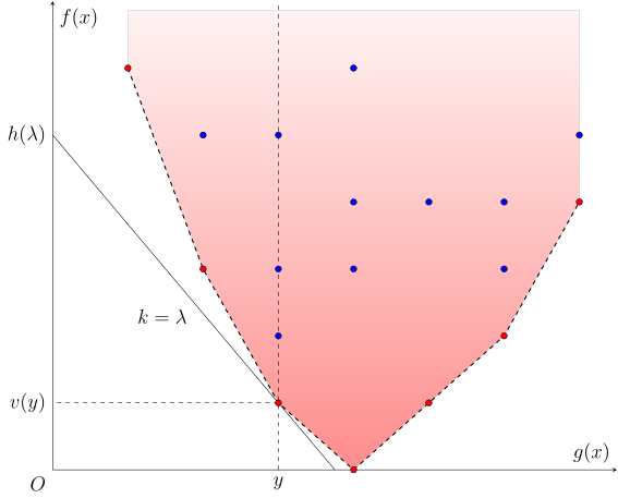
The red and blue points are the projections of all possible choices in $X$ onto the plane $(g(x),f(x))$ , forming $\mathcal D$ . The original problem asks for the smallest vertical coordinate among the points whose horizontal coordinate is $y$ , namely $v(y)$ . As $y$ changes, all points $(y,v(y))$ form the set of red points in the figure．

To obtain the vertical coordinate of $(y,v(y))$ , consider a line of slope $\lambda\in\mathbf R$ tangent to $\mathcal D$ . When the slope is appropriate, the line through $(y,v(y))$ has the smallest intercept $f(x)-\lambda g(x)$ among all lines of slope $\lambda$ passing through points of $\mathcal D$ . Let this minimum be

h(\lambda) = \min_{x\in X}f(x)-\lambda g(x).

Since $(y,v(y))$ also lies on this line, the solution of the original problem is

v(y) = h(\lambda) + \lambda y.

Suppose $h(\lambda)$ is easy to compute for every reasonable $\lambda$ . This is often true in contests because the original constraint has been removed. The two most important questions are then:

Does there exist a slope $\lambda$ whose minimum-intercept line passes through $(y,v(y))$ ?
If so, how can we find such a slope $\lambda$ ?

The first question is relatively easy. As the slope $\lambda$ changes, the set cut out by all these lines (the intersection of their corresponding upper half-planes) is necessarily convex. Therefore, these lines can pass through a point if and only if the point lies on the lower convex hull of this convex set. Equivalently, $v(y)$ is a convex function．

The second question is subtler. Since the desired point is known to have horizontal coordinate $y$ , a natural idea is to compute $g(x)$ at the current optimal solution $x_\lambda$ while computing $h(\lambda)$ . In the preceding example, when solving the penalized problem, record the number of selected items in an optimal solution. Compare $g(x_\lambda)$ with the desired $y$ , and adjust the next $\lambda$ interval accordingly. This is the most traditional WQS binary-search method．

In summary, the traditional WQS binary-search process is:

Initially, choose a reasonable interval for $\lambda$ ．
Choose a $\lambda$ in the current interval．
Solve $h(\lambda)=\min_{x\in X}f(x)-\lambda g(x)$ and record $g(x)$ at an optimal solution $x_\lambda$ , obtaining $g(x_\lambda)$ ．
If $g(x_\lambda)=y$ , the optimal value is $v(y)=h(\lambda)+\lambda y$ ; terminate．
Otherwise, adjust the interval for $\lambda$ according to the relation between $g(x_\lambda)$ and $y$ , then return to step 2．

This basic process is enough for some problems, but it is not complete. The improvements to it are discussed next．

Handling Collinear Cases

The first problem with the basic process is that it cannot handle collinear points correctly．

If three or more red points on the lower convex hull of $\mathcal D$ are collinear, the basic process may fail to compare $g(x_\lambda)$ and $y$ correctly. Suppose three collinear red points have horizontal coordinates $y_1,y_2,y_3$ and their common line has slope $\lambda^*$ . To compute $v(y_2)$ correctly, the last problem computed when the algorithm terminates must be $h(\lambda^*)$ , because $\lambda^*$ is the only slope of a minimum-intercept line that can pass through $(y_2,v(y_2))$ . However, while computing $h(\lambda^*)$ , the recorded value $g(x_{\lambda^*})$ may be any of $y_1,y_2,y_3$ . If the recorded $g(x_{\lambda^*})$ is not $y_2$ , the algorithm continues incorrectly and adjusts the $\lambda$ interval away from $y_2$ , eventually producing a wrong answer．

One way to handle collinearity is always to make $g(x_\lambda)$ as large as possible (or as small as possible) when recording the optimal solution $x_\lambda$ . At the same time, change the binary-search termination condition from finding $g(x_\lambda)=y$ for some $\lambda$ to finding the smallest (or largest) $\lambda$ satisfying $g(x_\lambda)\ge y$ (or $g(x_\lambda)\le y$ ). In the example above, this means that computing $h(\lambda^*)$ returns $g(x_{\lambda^*})$ equal to $y_3$ , ensuring that the last computed problem is $h(\lambda^*)$ . Note that the final output is $h(\lambda)+\lambda y$ , not $h(\lambda)+\lambda g(x_{\lambda})$ , because the recorded $g(x_\lambda)$ need not equal the actual constraint $y$ ．

Another approach is binary search over real numbers. If all numbers in the problem are integers, the slope in WQS binary search is clearly also an integer. Real-valued binary search is introduced so that if the correct choice $\lambda^*$ is accidentally discarded, the fractional part can move the search back toward it, ultimately approaching the correct answer $\lambda^*$ . For example, if the recorded $g(x_{\lambda^*})$ is $y_1$ , smaller than the desired $y_2$ , while computing $h(\lambda^*)$ , the algorithm considers $(\lambda^*,\lambda_r]$ , where $\lambda_r$ is the right endpoint of the current $\lambda$ interval. For integers, this should actually be $[\lambda_*+1,\lambda_r]$ , which rules out approaching $\lambda^*$ later. With real binary search, the interval remains $(\lambda^*,\lambda_r]$ ; for $\lambda$ in this interval, computing $h(\lambda)$ always records a value $g(x_\lambda)$ at least $y_3$ , strictly greater than $y_2$ . The right half is therefore repeatedly discarded as the algorithm proceeds, and the final range of $\lambda$ is guaranteed to lie near $\lambda^*$ . Since the desired slope is known to be an integer, the final precision need only ensure that the binary-search interval contains one integer; that integer is the desired $\lambda^*$ ．

After collinear cases are handled correctly, WQS binary search solves most WQS binary-search problems encountered in algorithm contests. However, it still cannot handle cases where $g(x_\lambda)$ is difficult to record, nor higher-dimensional cases with multiple coplanar points. We now examine the properties of the optimization problem $v(y)$ and give a more general method．

The Dual Method

This section presents a WQS binary-search implementation that only requires, for every $\lambda\in\mathbf R^d$ , efficient computation of

h(\lambda) = \min_{x\in X}f(x)-\lambda\cdot g(x)

the value, together with convexity of the original value function $v(y)$ over $y\in\mathbf R^d$ ¹. In one sentence, we prove that the value function $v(y)$ of the original problem equals the optimal value of its dual problem,

v^\star(y) = \sup_{\lambda\in\mathbf R^d} h(\lambda)+\lambda\cdot y,

and that the dual objective is concave in $\lambda\in\mathbf R^d$ , hence unimodal. It can therefore be solved efficiently by ternary search or golden-section search, with complexity still $O(T(n)\log^d L)$ . This completely resolves the problem of recording $g(x_\lambda)$ in the traditional method and allows WQS binary search to be applied in higher dimensions．

This section also shows that the range of $g(x_\lambda)$ can be obtained from $h(\lambda)$ without recording it separately while solving $h(\lambda)$ . For example, when $d=1$ and the problem involves only integers, the range of $g(x_\lambda)$ is exactly

[h(\lambda-1)-h(\lambda),h(\lambda)-h(\lambda+1)].

This provides another way to handle collinear cases in problems that must use the binary-search process described above．

The conclusions are proved using convex analysis. Specific applications can be found in the Example Problems section．

Lagrange Duality

Consider solving the problem with the Lagrange multiplier method. Introduce a Lagrange multiplier $\lambda\in\mathbf R^d$ . The Lagrangian is

L(x,\lambda,y) = f(x) - \lambda\cdot g(x)+\lambda\cdot y.

If any component of $g(x)-y$ is nonzero, the corresponding component of $\lambda$ can tend to positive or negative infinity, so

\sup_{\lambda\in\mathbf R^d}L(x,\lambda,y) = \begin{cases} f(x),&g(x)=y,\\ +\infty,&\text{otherwise}. \end{cases}

Thus the original problem can be written as

\begin{aligned} v(y) &= \min_{x\in X}\sup_{\lambda\in\mathbf R^d}L(x,\lambda,y). \end{aligned}

Exchanging the two optimization operations gives the dual problem:

\begin{aligned} v^\star(y)&=\sup_{\lambda\in\mathbf R^d}\min_{x\in X}L(x,\lambda,y)\\ &=\sup_{\lambda\in\mathbf R^d}h(\lambda)+\lambda\cdot y. \end{aligned}

We will show that under the condition that $v(y)$ is convex in $y$ , strong duality holds: $v^\star(y)=v(y)$ ．

Convex Conjugate

To establish strong duality, we need the notion of a convex conjugate．

Convex Conjugate

For a function $f:\mathbf R^d\rightarrow\mathbf R\cup\{\pm\infty\}$ , its convex conjugate, also called the Legendre–Fenchel transformation, is

f^*(x^*) = \sup_{x\in\mathbf R^d}x^*\cdot x - f(x).

Viewed as a function of $x^*$ , $f^*(x^*)$ is the supremum of a family of linear functions, so it is necessarily convex on $\mathbf R^d$ ．

“Slope Vector” and “Intercept” of a Hyperplane

Every hyperplane in the vector space $\mathbf R^{d+1}$ discussed here has the form

y = k\cdot x + b.

Thus, hyperplanes parallel to the $y$ -axis are not considered. For convenience, we informally call $k$ the “slope vector” and $b$ the “intercept” of the hyperplane. Writing the equation in standard form gives

k\cdot x - y = -b.

A normal vector is $(k,-1)$ . Thus, the so-called slope vector consists of the first $d$ components of the normal vector after normalizing its last component to $-1$ ．

Geometrically, the convex conjugate of $f(x)$ describes hyperplanes with slope vector $x^*$ that intersect the epigraph of the function $f(x)$

\operatorname{epi}f = \{(x,y)\in\mathbf R^d\times\mathbf R:f(x)\le y\}

of $f(x)$ . The minimum intercept $f(x)-x^*\cdot x$ among these hyperplanes is $-f^*(x^*)$ . In other words, $f(x)$ always lies above the hyperplane $y = x^*\cdot x-f^*(x^*)$ , and the hyperplane is tangent at $(x_0,f(x_0))$ , possibly with other tangent points. Such a hyperplane is a supporting hyperplane of $f(x)$ at $x_0$ . The intercept of a supporting hyperplane is uniquely determined by its slope vector, and the convex conjugate provides this mapping from slope vector to intercept．

Minimizing $f(x)-\lambda\cdot g(x)$ over $X$ is equivalent to minimizing $v(y)-\lambda\cdot y$ over $\{(y,v(y))\}$ :

\begin{aligned} \min_x f(x)-\lambda\cdot g(x) &= \min_{y\in g(X)}\left(\min_{x\in X:g(x)=y} f(x) - \lambda\cdot g(x)\right)\\ &= \min_{y\in g(X)}\left(\min_{x\in X:g(x)=y} f(x)\right) - \lambda\cdot y \\ &= \min_{y\in g(X)}v(y) - \lambda\cdot y. \end{aligned}

Therefore,

h(\lambda) = \min_{y\in g(X)}v(y) - \lambda\cdot y = -v^*(\lambda).

Thus $h(\lambda)$ is concave in $\lambda\in\mathbf R^d$ , and

v^\star(y) = \sup_{\lambda\in\mathbf R^d}\lambda\cdot y-v^*(\lambda) = v^{**}(y).

The value function $v^{\star}(y)$ of the dual problem is therefore the double convex conjugate of the original value function $v(y)$ , also called the biconjugate．

The problem becomes: which functions $v(y)$ equal their own biconjugate? The following theorem answers this．

Theorem (Fenchel–Moreau)

For $f:\mathbf R^d\rightarrow\mathbf R\cup\{\pm\infty\}$ , $f^{**}=f$ if and only if one of the following holds:

$f(x)$ is a proper convex function and lower semicontinuous;
$f(x)\equiv+\infty$ ; or
$f(x)\equiv-\infty$ ．

Proof

A function is proper if and only if it never takes the value $-\infty$ and is not identically $+\infty$ ．

For improper functions, one can verify that $f(x)\equiv+\infty$ and $f(x)\equiv-\infty$ are convex conjugates of one another. Apart from these, if $f(x)$ takes the value $-\infty$ at any point, then necessarily $f^*(x^*)\equiv+\infty$ . Thus these are the only improper functions satisfying $f^{**}=f$ . The rest of the proof concerns proper functions. For a proper function, lower semicontinuity and convexity are equivalent to its epigraph being a closed convex set．

Necessity is easy. Since $f=f^{**}$ is the convex conjugate of $f^*$ , it is the supremum of linear functions. The epigraph of $f(x)$ is therefore an intersection of closed convex sets and is itself closed and convex. Hence every proper function satisfying $f^{**}=f$ is lower semicontinuous and convex．

Conversely, these conditions are sufficient. As in other strong-duality proofs, divide the proof into two steps．

First prove weak duality, $f(x)\ge f^{**}(x)$ . By the definition of the convex conjugate, for all $x,x^*\in\mathbf R^d$ ,

f^*(x^*) \ge x^*\cdot x-f(x).

Therefore, for all $x,x^*\in\mathbf R^d$ ,

f(x) \ge x^*\cdot x-f^*(x^*).

Taking the supremum over $x^*$ on the right gives $f(x)\ge f^{**}(x)$ ．

Second, use the hyperplane separation theorem to show $f(x)\le f^{**}(x)$ . Suppose otherwise: for some $x_0\in\mathbf R^d$ , $f(x_0)>f^{**}(x_0)$ . Since the epigraph $\operatorname{epi}(f)$ is closed and convex and the singleton $\{(x_0,f^{**}(x_0))\}$ is compact and convex, the separation theorem gives $(\lambda,t)\in\mathbf R^d\times\mathbf R$ and $\alpha\in\mathbf R$ such that for every $x\in\operatorname{dom} f:=\{x\in\mathbf R^d:f(x)<+\infty\}$ and every $y\ge f(x)$ ,

\lambda\cdot x-ty <\alpha <\lambda\cdot x_0 - tf^{**}(x_0)

Since $y$ can be arbitrarily large, $t\ge 0$ . There are two cases．

First let $t>0$ . Divide through by $t$ , and set $\lambda'=t^{-1}\lambda$ and $\alpha'=t^{-1}\alpha$ :

\lambda'\cdot x-y < \alpha'< \lambda'\cdot x_0-f^{**}(x_0).

For every $x\in\operatorname{dom} f$ , set $y=f(x)$ to obtain

\alpha' > \lambda'\cdot x - f(x).

Taking the supremum over $x$ on the right gives

\alpha' \ge \sup_{x\in\mathbf R^d}\lambda'\cdot x - f(x) = f^*(\lambda').

Hence

f^{**}(x_0) < \lambda'\cdot x_0-f^*(\lambda') \le \sup_{x^*\in\mathbf R^d}x^*\cdot x_0-f^*(x^*) = f^{**}(x_0).

This contradiction rules out $t>0$ ．

Finally let $t=0$ . We show that a perturbation converts this into the $t>0$ case. Choose any $\lambda_0\in\operatorname{dom}f^*$ . By the definition of the convex conjugate, for every $x\in\operatorname{dom}f$ and $y\ge f(x)$ ,

\lambda_0\cdot x-y\le f^*(\lambda_0).

Therefore, for every $\varepsilon>0$ ,

(\lambda+\varepsilon\lambda_0)\cdot x - \varepsilon y<\alpha+\varepsilon f^*(\lambda_0).

Since $\alpha<\lambda\cdot x_0$ , for sufficiently small $\varepsilon>0$ we also have

\alpha+\varepsilon f^*(\lambda_0) < (\lambda+\varepsilon\lambda_0)\cdot x_0 - \varepsilon f^{**}(x_0).

Set $\lambda'=\lambda+\varepsilon\lambda_0$ , $t'=\varepsilon$ , and $\alpha'=\alpha+\varepsilon f^*(\lambda_0)$ . Then

\lambda'\cdot x-t'y <\alpha' <\lambda'\cdot x_0 - t'f^{**}(x_0).

This returns to the previous case and again gives a contradiction．

Therefore no $x_0\in\mathbf R^d$ satisfies $f(x_0)>f^{**}(x_0)$ , so $f(x_0)\le f^{**}(x_0)$ always. Combining the two steps gives $f^{**}(x)=f(x)$ ．

Therefore, strong duality holds if and only if $v(y)$ is convex in $y\in\mathbf R^d$ ²．

Subgradients

The previous section showed that the value function $h(\lambda)$ of the penalized problem is the negative of the convex conjugate of the original value function $v(y)$ . Since the definition of a convex conjugate is itself a parameterized optimization problem, a result similar to the envelope theorem also holds. However, convex functions are not differentiable everywhere, so the definition of a derivative must first be extended to convex functions. This leads to the notion of a subgradient．

Subgradient

For a convex function $f:\mathbf R^d\rightarrow\mathbf R\cup\{\pm\infty\}$ and $x_0\in\operatorname{dom}f$ , if $x^*\in\mathbf R^d$ satisfies

f(x) \ge f(x_0)+x^*\cdot(x-x_0),

for every $x\in\mathbf R^d$ , then $x^*$ is a subgradient of $f(x)$ at $x_0$ . The set of all subgradients of $f(x)$ at $x_0$ is its subdifferential, denoted $\partial f(x_0)$ ．

Geometrically, the subdifferential of a convex function $f(x)$ at $x_0$ is the set of slope vectors of all its supporting hyperplanes there. In one dimension,

\partial f(x_0) = [\partial_-f(x_0),\partial_+f(x_0)],

where $\partial_-f(x_0)$ and $\partial_+f(x_0)$ are the left and right derivatives of $f(x)$ at $x_0$ . For the extension $\tilde f(x)$ of a convex function $f:\mathbf Z\rightarrow\mathbf R\cup\{\pm\infty\}$ on the integers, its left and right derivatives at the integer point $x=k$ are the first differences on the two sides:

\partial\tilde f(k) = [f(k)-f(k-1),f(k+1)-f(k)].

Clearly, a convex function $f(x)$ is differentiable at $x_0$ if and only if its subdifferential $\partial f(x_0)$ is a singleton．

Because the convex conjugate maps slope vectors of supporting hyperplanes to their intercepts, it can determine whether a slope vector $x^*$ is a subgradient of $f(x)$ at a given point $x$ ．

Theorem (Convex Conjugates and Subgradients)

For a proper convex function $f:\mathbf R^d\rightarrow\mathbf R$ and any $x,x^*\in\mathbf R^d$ ,

x^*\in\partial f(x) \iff x^*\cdot x = f(x) + f^*(x^*).

If $f$ is also lower semicontinuous, these two conditions are also equivalent to $x\in\partial f^*(x^*)$ ．

Proof

By the definition of a subgradient, $x^*\in\partial f(x)$ if and only if

f(x') \ge f(x) + x^*\cdot(x'-x),~\forall x'\in\mathbf R^d.

This is equivalent to

x^*\cdot x - f(x) \ge x^*\cdot x'-f(x'),~\forall x'\in\mathbf R^d.

Equivalently,

x^*\cdot x - f(x) \ge \sup_{x'\in\mathbf R^d}x^*\cdot x'-f(x') = f^*(x^*).

By the definition of the convex conjugate, we always have

x^*\cdot x - f(x) \le f^*(x^*).

Thus the previous inequality is actually an equality, equivalently

x^*\cdot x = f(x) + f^*(x^*).

This proves the first part．

If $f$ is a lower-semicontinuous proper convex function, the Fenchel–Moreau theorem gives $f^{**}=f$ . Thus the two conditions are equivalent to

x^*\cdot x = f^*(x^*) + f^{**}(x).

Applying the first part again, they are equivalent to $x\in\partial f^*(x^*)$ ．

This result says that if $f^{**}=f$ , then the subdifferential $\partial f^{*}(x^*)$ of the convex conjugate $f^*$ at $x^*$ is exactly the set of $x$ -components of the intersections between the supporting hyperplanes with slope vector $x^*$ and the epigraph $\operatorname{epi}f$ ．

Corollary

For a lower-semicontinuous proper convex function $f:\mathbf R^d\rightarrow\mathbf R$ and any $x,x^*\in\mathbf R^d$ ,

\begin{aligned} \partial f(x) &= \arg\max_{y^*\in\mathbf R^d} x\cdot y^* - f^*(y^*),\\ \partial f^*(x^*) &= \arg\max_{y\in\mathbf R^d} x^*\cdot y - f(y). \end{aligned}

Proof

We prove the second equality; the first is similar．

By the definition of the convex conjugate,

f^*(x^*) = \sup_{y\in\mathbf R^d} x^*\cdot y - f(y),

x \in \arg\max_{y\in\mathbf R^d} x^*\cdot y - f(y)

if and only if $f^*(x^*) = x^*\cdot x - f(x)$ , and this equality holds if and only if $x\in\partial f^*(x^*)$ . Thus the two sets are equal．

In the setting of this article, this result says that when solving

h(\lambda) = \min_{x\in X}f(x)-\lambda\cdot g(x) = \min_{y\in g(X)}v(y) - \lambda\cdot y

the values of the constraint function $g(x)$ over the optimal decision set are exactly $\partial(-h(\lambda))$ . When $d=1$ and the problem involves only integers, this set is the interval

[h(\lambda-1)-h(\lambda),h(\lambda)-h(\lambda+1)].

For consecutive integer $\lambda$ , these intervals meet end to end, so binary search only needs to compute one endpoint．

Convexity Proofs

The prerequisite for WQS binary search is convexity of the value function. In contests, convexity can be guessed by tabulation or intuition, but a rigorous proof is often difficult. This section uses the following classic problem to introduce common ways of proving convexity in algorithm contests．

Planting Trees

There are $n$ tree pits, and $m$ trees must be planted. Trees cannot be planted in adjacent pits. Given a length- $n$ sequence $\{a_i\}$ representing the benefit of planting a tree in each pit, where benefits may be positive or negative, find the maximum possible total benefit of planting all $m$ trees．

In short, this is the problem of finding a maximum-weight independent set of size $m$ on a path of length $n$ ．

These methods can roughly be divided into four categories:

Prove convexity of the value function by reducing to a convex optimization problem (including linear programming), for example by constructing a min-cost flow model;
Prove convexity inductively from the state transition, possibly using convexity-preserving transformations;
For interval-partition problems, verify that each interval cost function satisfies the quadrangle inequality;
For special problems, establish convexity directly by an exchange argument．

These proof methods are often connected to a corresponding solution method for the problem．

Reduction to Parametric Convex Optimization

Consider the parametric convex optimization problem

v(y)=\inf_{x\in\mathcal D(y)} f(x,y).

The objective $f:\mathbf R^n\times\mathbf R^d\rightarrow\mathbf R\cup\{\pm\infty\}$ is convex in $x\in\mathbf R^m$ for every $y\in\mathbf R^d$ , while the feasible-set mapping $\mathcal D:\mathbf R^d\rightarrow \mathcal P(\mathbf R^m)$ is set-valued on $\mathbf R^d$ and has convex values $\mathcal D(y)$ for every $y\in\mathbf R^d$ . These conditions make this a convex optimization problem for every parameter $y\in\mathbf R^d$ ．

Theorem

Suppose the parametric convex optimization problem above satisfies:

The objective $f(x,y)$ is convex in $(x,y)$ ;
The graph $\{(x,y):x\in\mathcal D(y)\}$ of the feasible-set mapping $y\mapsto\mathcal D(y)$ is convex．

If $v(y)>-\infty$ for every $y\in\mathbf R^d$ , then the value function $v(y)$ is a proper convex function of $y$ ．

Proof

For any $y_1,y_2\in\mathbf R^d$ and $\alpha\in(0,1)$ , we need to prove

v(\alpha y_1+(1-\alpha)y_2) \le \alpha v(y_1) + (1-\alpha) v(y_2).

If $v(y_1)=+\infty$ or $v(y_2)=+\infty$ , the right-hand side is $+\infty$ and the inequality is immediate. Otherwise, $v(y_1)$ and $v(y_2)$ are both finite. For every $\varepsilon>0$ and $i=1,2$ , there exists $x_i\in\mathcal D(y_i)$ such that $f(x_i,y_i)< v(y_i)+\varepsilon$ . Convexity of the graph of $\mathcal D$ gives

\alpha x_1+(1-\alpha)x_2 \in \mathcal D(\alpha y_1+(1-\alpha)y_2).

Thus $\alpha x_1+(1-\alpha)x_2$ is feasible for the optimization problem with parameter $\alpha y_1+(1-\alpha)y_2$ . By optimality and convexity of the objective,

\begin{aligned} v(\alpha y_1+(1-\alpha)y_2) &\le f(\alpha x_1+(1-\alpha)x_2,\alpha y_1+(1-\alpha)y_2) \\ &\le \alpha f(x_1,y_1) + (1-\alpha)f(x_2,y_2) \\ &< \alpha v(y_1) + (1-\alpha) v(y_2) + \varepsilon. \end{aligned}

Since $\varepsilon$ is arbitrary, let $\varepsilon\rightarrow 0$ to obtain

v(\alpha y_1+(1-\alpha)y_2) \le \alpha v(y_1) + (1-\alpha) v(y_2).

Therefore the value function $v(y)$ is convex．

The most common convex optimization problems in algorithm contests are linear programs．

Corollary

Let $c\in\mathbf R^n$ , $A_1\in\mathbf R^{d_1\times n}$ , $A_2\in\mathbf R^{d_2\times n}$ , $y_1\in\mathbf R^{d_1}$ , and $y_2\in\mathbf R^{d_2}$ . Consider the parametric linear program

v(y_1,y_2)=\min_{x\in\mathbf R^n} c\cdot x \text{ subject to }A_1x\le y_1,A_2x=y_2,x\ge 0.

Then the value function $v(y_1,y_2)$ is convex in $(y_1,y_2)$ ．

Whether the constraints are inequalities or equalities, the value function of a linear program is convex in the parameters of the constraints．

Many graph problems can be written as linear programs:

Network-flow problems: maximum flow, minimum cut, and minimum-cost flow;
Shortest paths with no negative cycles;
Maximum (weight) matching and minimum vertex cover in bipartite graphs;
Maximum (weight) matching in general graphs;
Minimum spanning tree³．

Therefore, the value functions of these problems are convex (or concave) functions of their parameters．

Integer Constraints

When graph models are used to model real problems, implicit integer constraints often exist, such as an edge being either selected or not selected and flow being integral. Thus they become integer linear programs (integer linear programming, ILP), rather than linear programs (LP). Since ILP is not a convex optimization problem, its value function need not be convex in the problem parameters. Relaxing the integer constraints in an ILP gives an LP, but the latter need not have an optimal solution satisfying the integer constraints. Therefore, the optimal value of the relaxed LP may be strictly better than that of the corresponding ILP, and the two need not be equivalent．

The graph problems listed above can all be written as LPs without integer constraints. For other problems, such as maximum independent set in a general graph, integer constraints are necessary. Moreover, even if a graph problem can be written as an LP, adding extra linear constraints may destroy the equivalence between the corresponding ILP and LP, so the constrained graph problem may no longer have an LP formulation．

For example, in the context of min-cost flow, we have the following familiar result:

Corollary

In the min-cost flow model, the minimum cost $v(m)$ is a convex function of the flow $m$ ．

Proof

Let $G=(V,E)$ be a directed graph. Let edge $(i,j)$ have capacity $c_{ij}$ and per-unit cost $w_{ij}$ , with source $s$ and sink $t$ . Let the decision variables be $\{f_{ij}\}$ , where $f_{ij}$ is the flow on edge $(i,j)\in E$ . The min-cost flow can be written as the linear program

\begin{aligned} v(m)=\min_{\{f_{ij}\}}\;&\sum_{(i,j)\in E}w_{ij}f_{ij}\\ \text{subject to }&\sum_{(j,i)\in E}f_{ji} - \sum_{(i,j)\in E}f_{ij} = \begin{cases} -m, & i=s,\\ m, & i=t,\\ 0, & \text{otherwise}, \end{cases} ~\forall i\in V,\\ &0\le f_{ij}\le c_{ij},~\forall (i,j)\in E. \end{aligned}

Thus the minimum cost $v(m)$ is convex in the parameter $m$ ．

Many problems in algorithm contests can be reduced to network flow or other graph problems, and their value-function convexity can be proved similarly．

This method gives the first convexity proof for the tree-planting problem:

Convexity Proof 1

The maximum benefit in the tree-planting problem can be obtained from the following maximum-cost maximum-flow model:

From source $s$ , add an edge to vertex $r$ with capacity $m$ and cost $0$ ;
From vertex $r$ , add an edge of capacity $1$ and cost $0$ to every odd vertex $i=1,3,\cdots,2\lceil n/2\rceil-1$ ;
From every even vertex $i=0,2,\cdots,2\lfloor n/2\rfloor$ , add an edge of capacity $1$ and cost $0$ to sink $t$ ;
For each $i=1,\cdots,n$ , add an edge of capacity $1$ and cost $a_i$ from the odd vertex among $i-1$ and $i$ to the even vertex．

The final answer is the maximum cost found. Converting this graph model into the corresponding linear program (see the proof of the corollary above), the total flow $m$ appears in the inequality representing the flow constraint on edge $(s,r)$ . The corollary shows that the maximum cost $v(m)$ is concave in the flow $m$ ．

Using this cost-flow model, the problem can be solved in $O(n\log n)$ time by simulating cost flow or using regretful greedy．

Using the State Transition

Although a state transition may not provide an effective way to compute the answer, it can often prove that the state function $f(i,j)$ is convex in the parameter $j$ . Specifically, regard $f(i,\cdot)$ as the state at $i$ , and view the transition for $f(i,j)$ as a recurrence for $f(i,\cdot)$ . Convexity of every $f(i,\cdot)$ can then be proved inductively. This method is especially common in Slope Trick DP optimization, which also discusses common convexity-preserving transformations．

The same method proves convexity for the tree-planting problem:

Convexity Proof 2

Let $f(i,j)$ be the maximum benefit when $j$ trees are planted in the first $i$ pits. Consider

f(i,j) = \max\{f(i-1,j),f(i-2,j-1)+a_i\}.

View this transition as a recurrence for $f(i,\cdot)$ . Because the maximum involves two different functions, it cannot be expressed as a supremal convolution. Nevertheless, induction can still prove that $f(i,\cdot)$ is concave．

Specifically, prove inductively that:

$f(i,j)-f(i-2,j-1)$ is decreasing in $j$ ;
$f(i,j)-f(i-1,j)$ is increasing in $j$ ．

The induction base is trivial. Assume these statements hold for all $i-1$ and earlier indices; now prove them for $i$ . Direct verification is enough．

First, by the induction hypothesis,

f(i-1,j) - f(i-2,j-1) = (f(i,j)-f(i-2,j-1)) - (f(i,j)-f(i-1,j))

is decreasing in $j$ . Therefore,

f(i,j) - f(i-2,j-1) = \max\{f(i-1,j) - f(i-2,j-1), a_i\}

is decreasing in $j$ , and

f(i,j) - f(i-1,j) = \max\{0,a_i-(f(i,j) - f(i-2,j-1))\}

is increasing in $j$ . This completes the induction．

Consequently,

f(i,j) - f(i,j-1) = (f(i,j)-f(i-2,j-1)) - (f(i,j-1) - f(i-1,j-1)) - (f(i-1,j-1) - f(i-2,j-1))

is decreasing in $j$ . Thus $f(i,j)$ is concave in $j$ , and the value function $v(m)=f(n,m)$ is concave in $m$ ．

One by-product of this proof is that for every $i$ there is a $p_i$ such that

f(i,j) = \begin{cases} f(i-1,j), & j\le p_i,\\ f(i-2,j-1) + a_i, & j> p_i. \end{cases}

This means that the sequence $f(i,\cdot)$ can be maintained directly with a balanced tree in $O(n\log^2n)$ time. The benefit is that arbitrary tree-spacing conditions can be handled and all values of $v(m)$ are obtained at once．

Quadrangle Inequality

Another common class of problems with convex value functions in algorithm contests is interval partitioning. That page proves that if the cost function of a single interval satisfies the quadrangle inequality, then the minimum cost of an interval partition with a bounded number of intervals is convex in the number of intervals. It also gives methods for determining whether a function $w(l,r)$ satisfies the quadrangle inequality. The most direct method is to compute its mixed second difference:

\begin{aligned} \Delta_l \Delta_r w(l,r) &= \Delta_l(w(l,r+1)-w(l,r)) \\ &= w(l+1,r+1)-w(l+1,r)-w(l,r+1)+w(l,r). \end{aligned}

The function $w(l,r)$ satisfies the quadrangle inequality if and only if $\Delta_l \Delta_r w(l,r)$ is nonpositive. Intuitively, this usually means that expanding an interval in both directions—moving the left endpoint left and the right endpoint right—has some synergistic effect．

The tree-planting problem can also be viewed as interval partitioning, so its convexity can be proved by verifying the quadrangle inequality．

Convexity Proof 3

Add an arbitrary $a_0$ before the tree-benefit sequence. The tree-planting problem is then equivalent to partitioning $\{a_0,a_1,\cdots,a_n\}$ into $m$ segments, where the benefit function of each segment is

w(l,r) = \max_{i\in[l+1,r]} a_i

This is an interval-partition problem. The benefit of each segment is the maximum benefit of the trees other than the first tree, which guarantees that planted trees are separated．

Because this is a maximization problem, verify “crossing greater than containment”: for every a

w(a,c)+w(b,d) \ge w(a,d)+w(b,c).

Substitute the benefit function and set

A = \max_{i\in[a+1,b]} a_i,~ B = \max_{i\in[b+1,c]} a_i,~ C = \max_{i\in[c+1,d]}a_i,

The desired inequality becomes

\max\{A,B\} + \max\{B,C\} \ge \max\{A,B,C\} + B.

The larger of $\max\{A,B\}$ and $\max\{B,C\}$ on the left is $\max\{A,B,C\}$ , while the smaller is always at least $B$ , so the inequality holds．

After converting the tree-planting problem into interval partitioning, precompute interval extrema with an ST table or similar method. Then a single interval cost can be computed in $O(1)$ , and the interval-partition algorithm solves the problem in $O(n\log n\log L)$ or $O(n(n+m))$ time. The method also handles arbitrary tree-spacing conditions．

Exchange Argument

An exchange argument is often used to prove convexity of value functions in combinatorial optimization problems. Specifically, start from optimal solutions for parameters $m-1$ and $m+1$ , exchange some elements to construct a feasible solution for parameter $m$ with value at most $(v(m-1)+v(m+1))/2$ , and use optimality of $v(m)$ to prove convexity. Unlike convex optimization, combinatorial optimization has no natural way to construct an intermediate form of two solutions, so exchange arguments usually require some ingenuity．

“Increasing Marginal Cost” Does Not Necessarily Imply Convexity

Objective functions in combinatorial optimization often have increasing-marginal-cost properties, but this does not necessarily imply convexity. A typical example is [IOI 2005] River: its path version satisfies the quadrangle inequality and is therefore convex, but the tree version has cases where convexity fails．

A common property characterizing increasing marginal cost is supermodularity. For a function $f:\mathcal PX\rightarrow\mathbf R$ on the family of subsets $\mathcal PX$ of a finite set $X$ , if it satisfies either of the following equivalent properties:

(Crossing less than containment) For all subsets $A,B\subseteq X$ , $f(A)+f(B) \le f(A\cup B) + f(A\cap B)$ ;
(Increasing marginal cost) For all $A\subseteq B\subseteq X$ and $x\in X\setminus B$ , $f(A\cup\{x\})-f(A)\le f(B\cup\{x\})-f(B)$ ;

then $f$ is supermodular. However, in an optimization problem with a supermodular objective, the value function

v(m) = \min_{A\subseteq X} f(A) \text{ subject to }|A|=m

need not be convex in $m$ . The reason is that optimal solutions for subset sizes $m-1$ and $m+1$ generally cannot be used to construct a feasible subset of size $m$ satisfying the required value relation．

The exchange argument provides another proof of convexity for the tree-planting problem．

Convexity Proof 4

Use an exchange argument. Let optimal solutions for planting $m-1$ and $m+1$ trees be $\{x_i^{(m-1)}\}\in\{0,1\}^n$ and $\{x_i^{(m+1)}\}\in\{0,1\}^n$ , respectively. A value of $1$ means a tree is planted in the pit, and $0$ means no tree is planted. Define $\{z_i\}\in\{0,\pm 1\}^n$ by

z_i = x_i^{(m+1)} - x_i^{(m-1)},~i=1,\cdots,n.

This sequence marks the differences between the two planting schemes. A value of $0$ means that the pit either has a tree in both schemes or has no tree in either; $-1$ and $+1$ mean that the pit has a tree only in $x^{(m-1)}$ or only in $x^{(m+1)}$ , respectively. Since no scheme plants trees in adjacent pits:

In every consecutive nonzero segment, the values of $z_i$ alternate between $\pm 1$ ;
The $0$ values immediately outside a maximal consecutive nonzero segment mean that neither scheme plants a tree there．

If the sum of $z_i$ over a maximal consecutive nonzero segment is $+1$ , then scheme $x^{(m+1)}$ plants one more tree than scheme $x^{(m-1)}$ in that segment, so we can exchange the planting positions of the two schemes within the segment. This produces two feasible schemes, each planting $m$ trees. The total planting positions and count across the two schemes are unchanged, only redistributed, so their total benefit remains $v(m-1)+v(m+1)$ . These two $m$ -tree schemes need not be optimal, so each has benefit at most $v(m)$ . Hence

v(m-1) + v(m+1) \le 2v(m),

which means $v(m)$ is concave in $m$ ．

It remains to show that a maximal consecutive nonzero segment with sum $+1$ exists. Since it is a sum of alternating $\pm 1$ , the sum of each such segment is $0$ or $\pm 1$ . The sum of all maximal consecutive nonzero segments is $2$ , so at least two segments have sum exactly $+1$ . This completes the proof．

Example Problems

This section presents examples applying WQS binary search in different settings．

Template Problem

Luogu P1484 Planting Trees

There are $n$ tree pits, and at most $m$ trees may be planted. Trees cannot be planted in adjacent pits. Given a length- $n$ sequence $\{a_i\}$ representing the benefit of planting in each pit, where benefits may be positive or negative, find the maximum possible total benefit of planting these $m$ trees．

Solution

Unlike the tree-planting problem discussed above, this problem asks for at most $m$ trees rather than exactly $m$ . Let $v(m)$ still denote the value function of the earlier problem. The answer here is $\tilde v(m)=\max_{k\le m}v(k)$ . Since $v(m)$ is concave, hence unimodal, the answer keeps only the part of $v(m)$ rising to its peak and then remains at the peak. Equivalently, it retains only the part with nonnegative tangent slope. Thus the only difference from the earlier problem is that the initial slope range for WQS binary search is $[0,\max_ia_i]$ rather than $[\min_ia_i,\max_ia_i]$ ． After WQS binary search removes the cardinality constraint, the problem becomes maximum-weight independent set on a path, with the original profits $\{a_i\}$ replaced by $\{a_i+k\}$ . This is a classic dynamic programming problem. Let $f(i,j)$ be the maximum profit of the subproblem on the first $i$ pits when the $j=1$ state means planting and the $j=0$ state means leaving the $i$ -th pit empty. The transition is

\begin{aligned} f(i,0) &= \max\{f(i-1,0),f(i-1,1)\},\\ f(i,1) &= f(i-1,0) + a_i + k. \end{aligned}

The initial conditions are $f(0,0)=0$ and $f(0,1)=-\infty$ , and the final answer is $\max\{f(n,0),f(n,1)\}$ . One computation takes $O(n)$ time, so the total complexity is $O(n\log L)$ , where $L=\max_i|a_i|$ .

A reference implementation follows:

Traditional method

#include <algorithm>
#include <cstring>
#include <iostream>
#include <tuple>
#include <vector>

int main() {
  int n, m;
  std::cin >> n >> m;
  std::vector<int> a(n + 1);
  for (int i = 1; i <= n; ++i) std::cin >> a[i];
  // Calculate h(k) = max_x f(x) - k * g(x).
  // Meanwhile, obtain the maximum value g(x) of the optimizer x.
  auto calc = [&](int k) -> std::pair<long long, int> {
    long long dp[2] = {0, -0x3f3f3f3f3f3f3f3f};
    int opt[2] = {0, 0};
    for (int i = 1; i <= n; ++i) {
      long long tmp_dp[2];
      int tmp_opt[2];
      if (dp[0] > dp[1]) {
        tmp_dp[0] = dp[0];
        tmp_opt[0] = opt[0];
      } else if (dp[1] > dp[0]) {
        tmp_dp[0] = dp[1];
        tmp_opt[0] = opt[1];
      } else {
        tmp_dp[0] = dp[0];
        tmp_opt[0] = std::max(opt[0], opt[1]);
      }
      tmp_dp[1] = dp[0] + a[i] - k;
      tmp_opt[1] = opt[0] + 1;
      std::memcpy(dp, tmp_dp, sizeof(dp));
      std::memcpy(opt, tmp_opt, sizeof(opt));
    }
    long long val;
    int opt_m;
    if (dp[0] > dp[1]) {
      val = dp[0];
      opt_m = opt[0];
    } else if (dp[1] > dp[0]) {
      val = dp[1];
      opt_m = opt[1];
    } else {
      val = dp[0];
      opt_m = std::max(opt[0], opt[1]);
    }
    return {val, opt_m};
  };
  // WQS binary search.
  long long val, tar_val;
  int opt_m, tar_k;
  std::tie(val, opt_m) = calc(0);
  if (opt_m <= m) {
    // Have already reached the peak.
    tar_k = 0;
    tar_val = val;
  } else {
    // Find the maximum k such that g(x) >= m.
    int ll = 0, rr = 1000000;
    while (ll <= rr) {
      int mm = (ll + rr) / 2;
      std::tie(val, opt_m) = calc(mm);
      if (opt_m >= m) {
        tar_k = mm;
        tar_val = val;
        ll = mm + 1;
      } else {
        rr = mm - 1;
      }
    }
  }
  long long res = tar_val + (long long)tar_k * m;
  std::cout << res << std::endl;
  return 0;
}

Dual method

#include <algorithm>
#include <iostream>
#include <tuple>
#include <type_traits>
#include <vector>

// Golden section search on integer domain (unimodal function)
template <typename T, typename F>
typename std::enable_if<
    std::is_integral<T>::value,
    std::pair<T, decltype(std::declval<F>()(std::declval<T>()))>>::type
golden_section_search(T ll, T rr, F func) {
  constexpr long double phi = 0.618033988749894848204586834L;
  T ml = ll + static_cast<T>((rr - ll) * (1 - phi));
  T mr = ll + static_cast<T>((rr - ll) * phi);
  auto fl = func(ml), fr = func(mr);
  while (ml < mr) {
    if (fl > fr) {
      rr = mr;
      mr = ml;
      fr = fl;
      ml = ll + static_cast<T>((rr - ll) * (1 - phi));
      fl = func(ml);
    } else {
      ll = ml;
      ml = mr;
      fl = fr;
      mr = ll + static_cast<T>((rr - ll) * phi);
      fr = func(mr);
    }
  }
  T best_x = ll;
  auto best_val = func(ll);
  for (T i = ll + 1; i <= rr; ++i) {
    auto val = func(i);
    if (val > best_val) {
      best_val = val;
      best_x = i;
    }
  }
  return {best_x, best_val};
}

int main() {
  int n, m;
  std::cin >> n >> m;
  std::vector<int> a(n + 1);
  for (int i = 1; i <= n; ++i) std::cin >> a[i];
  // Calculate h(k) = max_x f(x) + k * g(x).
  auto calc = [&](int k) -> long long {
    long long dp[2] = {0, -0x3f3f3f3f3f3f3f3f};
    for (int i = 1; i <= n; ++i) {
      std::tie(dp[0], dp[1]) =
          std::make_pair(std::max(dp[0], dp[1]), dp[0] + a[i] + k);
    }
    return std::max(dp[0], dp[1]);
  };
  // Solve the dual problem to find v(m).
  // Implemented as a minimization problem by adding negative signs.
  // Only consider tangent lines of negative slopes to ignore the part
  //     of the curve after the peak.
  auto res = -golden_section_search(-1000000, 0, [&](int k) -> long long {
                return -calc(k) + (long long)k * m;
              }).second;
  std::cout << res << std::endl;
  return 0;
}

Luogu P2619 [National Training Team] Tree I

Given a weighted undirected connected graph whose edges are black or white, find the minimum-weight spanning tree containing exactly $m$ white edges.

Solution

First, an exchange argument proves that $v(m)$ is convex. Assume without loss of generality that all edge weights are distinct. Cases in which two edge weights are equal can be perturbed so that all edge weights become distinct; letting the perturbation tend to zero then shows that convexity still holds in the limiting case, namely when two edge weights are equal. The key to the proof is the following lemma:⁴

Lemma

Let $S$ and $T$ be two spanning trees of the undirected connected graph $G=(V,E)$ . For any $e\in S\setminus T$ , there exists at least one edge $f\in T\setminus S$ such that both $S-e+f$ and $T-f+e$ are spanning trees of $G$ .

Proof

Let $e=(u,v)$ , and let $P$ be the unique path in tree $T$ connecting $u$ and $v$ . Since $P+e$ is the unique cycle in $T+e$ , deleting any edge on $P$ , say $f$ , makes $T-f+e$ a spanning tree. Meanwhile, $S-e$ is a forest with two connected components, whose vertex sets are $V_1$ and $V_2$ . Therefore, choosing an edge $f\in P$ such that the edge $f$ connects $V_1$ and $V_2$ guarantees that $S-e+f$ is a spanning tree. Such an edge $f$ always exists because $u$ and $v$ belong to $V_1$ and $V_2$ , respectively, and $P$ connects $u$ and $v$ . Moreover, $f\notin S$ , because in $S-e$ , $V_1$ and $V_2$ are disconnected. This completes the proof.

Let $T_{m-1}$ and $T_{m+1}$ be minimum spanning trees with $m-1$ and $m+1$ white edges, respectively. Let $e$ be a white edge in $T_{m+1}\setminus T_{m-1}$ . Applying the lemma shows that there exists an edge $f\in T_{m-1}\setminus T_{m+1}$ such that $T'=T_{m+1}-e+f$ and $T''=T_{m-1}+e-f$ are both spanning trees. Since only one pair of edges is exchanged, the sum of the edge weights of $T'$ and $T''$ remains $v(m-1)+v(m+1)$ . We now consider two cases:

If $f$ is a black edge, then both $T'$ and $T''$ have $m$ white edges. The edge-weight sum of each is at least $v(m)$ . This proves $2v(m)\le v(m-1)+v(m+1)$ , and hence $v(m)$ is convex as a function of $m$ .
If $f$ is a white edge, then $T'$ and $T''$ have $m+1$ and $m-1$ white edges, respectively, so their edge-weight sums are at least $v(m+1)$ and $v(m-1)$ , respectively. However, we already know that their sums equal $v(m-1)+v(m+1)$ . This implies that the edge-weight sum of $T'$ is exactly $v(m+1)$ . Comparing $T'$ with $T_{m+1}$ shows that $e$ and $f$ must have equal weights. This contradicts the assumption, so this case cannot occur.

This proves that $v(m)$ is convex as a function of $m$ .

Once the convexity of $v(m)$ has been established, the problem can be solved with WQS binary search. Remove the cardinality constraint, subtract $k$ from the weight of every white edge, and solve the minimum spanning tree problem. For this, apply Kruskal's algorithm. Using a disjoint-set union to maintain connectivity, the complexity is $O(E\log E+E\alpha(V))$ , where $E$ and $V$ are the numbers of edges and vertices, respectively, and $\alpha(\cdot)$ is the inverse Ackermann function. The main part of the complexity, $O(E\log E)$ , is the cost of sorting the edges, and it can be optimized further in this problem. Although the WQS binary search requires computing a minimum spanning tree multiple times, only the weights of white edges are shifted by the same amount each time. Therefore, we can sort the white and black edges separately during preprocessing, and when computing each minimum spanning tree, we only need to merge the white and black edges after adjusting their weights. This reduces the total complexity to $O(E\log E+E\alpha(V)\log L)$ , where $L$ is the length of the range of possible edge weights.

A reference implementation follows:

Traditional method

#include <algorithm>
#include <array>
#include <iostream>
#include <numeric>
#include <tuple>
#include <vector>

class DisjointSet {
  std::vector<int> fa, sz;

  int find(int x) { return fa[x] == x ? x : fa[x] = find(fa[x]); }

 public:
  DisjointSet(int n) : fa(n), sz(n, 1) { std::iota(fa.begin(), fa.end(), 0); }

  bool unite(int x, int y) {
    x = find(x);
    y = find(y);
    if (x == y) return false;
    if (sz[x] < sz[y]) std::swap(x, y);
    fa[y] = x;
    sz[x] += sz[y];
    return true;
  }
};

int main() {
  int V, E, m;
  std::cin >> V >> E >> m;
  std::array<std::vector<std::array<int, 3>>, 2> edges;
  edges[0].reserve(E);  // white edges.
  edges[1].reserve(E);  // black edges.
  for (int i = 0; i < E; ++i) {
    int u, v, c, w;
    std::cin >> u >> v >> w >> c;
    edges[c].push_back({u, v, w});
  }
  // Sort edges.
  std::sort(edges[0].begin(), edges[0].end(),
            [&](const auto& lhs, const auto& rhs) -> bool {
              return lhs[2] < rhs[2];
            });
  std::sort(edges[1].begin(), edges[1].end(),
            [&](const auto& lhs, const auto& rhs) -> bool {
              return lhs[2] < rhs[2];
            });
  // Calculate h(k) = min_x f(x) - k * g(x) by Kruskal algorithm.
  // Use white edges first, whenever possible.
  auto calc = [&](int k) -> std::pair<int, int> {
    int res = 0, cnt = 0;
    DisjointSet djs(V);
    int i[2] = {};
    while (i[0] < edges[0].size() && i[1] < edges[1].size()) {
      int c = edges[0][i[0]][2] - k > edges[1][i[1]][2];
      if (djs.unite(edges[c][i[c]][0], edges[c][i[c]][1])) {
        res += edges[c][i[c]][2] - (c ? 0 : k);
        cnt += c ? 0 : 1;
      }
      ++i[c];
    }
    while (i[0] < edges[0].size()) {
      if (djs.unite(edges[0][i[0]][0], edges[0][i[0]][1])) {
        res += edges[0][i[0]][2] - k;
        ++cnt;
      }
      ++i[0];
    }
    while (i[1] < edges[1].size()) {
      if (djs.unite(edges[1][i[1]][0], edges[1][i[1]][1])) {
        res += edges[1][i[1]][2];
      }
      ++i[1];
    }
    return {res, cnt};
  };
  // WQS binary search.
  // Find the minimum k such that g(x) >= m.
  int val, opt_m, tar_val, tar_k;
  int ll = -100, rr = 100;
  while (ll <= rr) {
    int mm = ll + (rr - ll) / 2;
    std::tie(val, opt_m) = calc(mm);
    if (opt_m >= m) {
      tar_val = val;
      tar_k = mm;
      rr = mm - 1;
    } else {
      ll = mm + 1;
    }
  }
  int res = tar_val + tar_k * m;
  std::cout << res << std::endl;
  return 0;
}

Dual method

#include <algorithm>
#include <array>
#include <iostream>
#include <numeric>
#include <tuple>
#include <type_traits>
#include <vector>

// Golden section search on integer domain (unimodal function)
template <typename T, typename F>
typename std::enable_if<
    std::is_integral<T>::value,
    std::pair<T, decltype(std::declval<F>()(std::declval<T>()))>>::type
golden_section_search(T ll, T rr, F func) {
  constexpr long double phi = 0.618033988749894848204586834L;
  T ml = ll + static_cast<T>((rr - ll) * (1 - phi));
  T mr = ll + static_cast<T>((rr - ll) * phi);
  auto fl = func(ml), fr = func(mr);
  while (ml < mr) {
    if (fl > fr) {
      rr = mr;
      mr = ml;
      fr = fl;
      ml = ll + static_cast<T>((rr - ll) * (1 - phi));
      fl = func(ml);
    } else {
      ll = ml;
      ml = mr;
      fl = fr;
      mr = ll + static_cast<T>((rr - ll) * phi);
      fr = func(mr);
    }
  }
  T best_x = ll;
  auto best_val = func(ll);
  for (T i = ll + 1; i <= rr; ++i) {
    auto val = func(i);
    if (val > best_val) {
      best_val = val;
      best_x = i;
    }
  }
  return {best_x, best_val};
}

class DisjointSet {
  std::vector<int> fa, sz;

  int find(int x) { return fa[x] == x ? x : fa[x] = find(fa[x]); }

 public:
  DisjointSet(int n) : fa(n), sz(n, 1) { std::iota(fa.begin(), fa.end(), 0); }

  bool unite(int x, int y) {
    x = find(x);
    y = find(y);
    if (x == y) return false;
    if (sz[x] < sz[y]) std::swap(x, y);
    fa[y] = x;
    sz[x] += sz[y];
    return true;
  }
};

int main() {
  int V, E, m;
  std::cin >> V >> E >> m;
  std::array<std::vector<std::array<int, 3>>, 2> edges;
  edges[0].reserve(E);  // white edges.
  edges[1].reserve(E);  // black edges.
  for (int i = 0; i < E; ++i) {
    int u, v, c, w;
    std::cin >> u >> v >> w >> c;
    edges[c].push_back({u, v, w});
  }
  // Sort edges.
  std::sort(edges[0].begin(), edges[0].end(),
            [&](const auto& lhs, const auto& rhs) -> bool {
              return lhs[2] < rhs[2];
            });
  std::sort(edges[1].begin(), edges[1].end(),
            [&](const auto& lhs, const auto& rhs) -> bool {
              return lhs[2] < rhs[2];
            });
  // Calculate h(k) = min_x f(x) - k * g(x) by Kruskal algorithm.
  auto calc = [&](int k) -> int {
    int res = 0;
    DisjointSet djs(V);
    int i[2] = {};
    while (i[0] < edges[0].size() && i[1] < edges[1].size()) {
      int c = edges[0][i[0]][2] - k > edges[1][i[1]][2];
      if (djs.unite(edges[c][i[c]][0], edges[c][i[c]][1])) {
        res += edges[c][i[c]][2] - (c ? 0 : k);
      }
      ++i[c];
    }
    while (i[0] < edges[0].size()) {
      if (djs.unite(edges[0][i[0]][0], edges[0][i[0]][1])) {
        res += edges[0][i[0]][2] - k;
      }
      ++i[0];
    }
    while (i[1] < edges[1].size()) {
      if (djs.unite(edges[1][i[1]][0], edges[1][i[1]][1])) {
        res += edges[1][i[1]][2];
      }
      ++i[1];
    }
    return res;
  };
  // Solve the dual problem to find v(m).
  auto res = golden_section_search(-100, 100, [&](int k) -> int {
               return calc(k) + k * m;
             }).second;
  std::cout << res << std::endl;
  return 0;
}

Interval Partition Problem

Luogu P6246 [IOI 2000] Enhanced Post Office Enhanced

Given an increasing sequence of $n$ positive integers $\{a_i\}$ representing the positions of $n$ villages beside a highway, build $m$ post offices. The positions of the post offices should be chosen to minimize the sum of the distances from all villages to their nearest post office. Find this minimum.

Solution

This is a typical interval partition problem. See that page for implementation details of the monotone queue.

Each post office serves the villages closest to it, which must form a contiguous block along the highway. Building $m$ post offices is therefore equivalent to partitioning the villages into $m$ contiguous segments and building the cheapest possible post office for each segment. The post office for a segment should be placed at the median village. Thus the cost function for $[l,r]$ is

w(l,r) = \sum_{i=l}^r|a_i-a_{\lfloor(l+r)/2\rfloor}|.

It satisfies the quadrangle inequality because its mixed second difference is nonpositive:

\Delta_l\Delta_r w(l,r) = \Delta_l(a_{r+1} - a_{\lfloor(l+r+1)/2\rfloor}) = a_{\lfloor(l+r+1)/2\rfloor}-a_{\lfloor(l+r+2)/2\rfloor} \le 0.

Therefore, combining a monotone queue with WQS binary search solves the problem in $O(n\log n\log L)$ time.

A reference implementation follows:

Traditional method

#include <cmath>
#include <deque>
#include <iostream>
#include <tuple>
#include <type_traits>
#include <vector>

// Monotone decision DP.
// This solves f(i) = min f(j-1) + w(j,i) s.t. 1 <= j <= i.
// Also records the minimal optimal decision j for each f(i).
template <typename W>
std::pair<std::vector<decltype(std::declval<W>()(0, 0))>, std::vector<int>>
monotone_decision_opt_dp(int n, W ww) {
  using ValueT = decltype(std::declval<W>()(0, 0));
  std::vector<ValueT> f(n + 1);
  std::vector<int> opt(n + 1), lt(n + 1), rt(n + 1);
  std::deque<int> dq;
  auto w = [&](int j, int i) -> ValueT { return ww(j, i) + f[j - 1]; };
  for (int j = 1; j <= n; ++j) {
    if (!dq.empty() && rt[dq.front()] < j) dq.pop_front();
    if (!dq.empty()) lt[dq.front()] = j;
    while (!dq.empty() && w(j, lt[dq.back()]) < w(dq.back(), lt[dq.back()])) {
      dq.pop_back();
    }
    if (dq.empty()) {
      lt[j] = j;
      rt[j] = n;
      dq.emplace_back(j);
    } else if (w(j, rt[dq.back()]) >= w(dq.back(), rt[dq.back()])) {
      if (rt[dq.back()] < n) {
        lt[j] = rt[dq.back()] + 1;
        rt[j] = n;
        dq.emplace_back(j);
      }
    } else {
      int ll = lt[dq.back()], rr = rt[dq.back()], i = rr;
      while (ll <= rr) {
        int mm = (ll + rr) / 2;
        if (w(j, mm) < w(dq.back(), mm)) {
          i = mm;
          rr = mm - 1;
        } else {
          ll = mm + 1;
        }
      }
      rt[dq.back()] = i - 1;
      lt[j] = i;
      rt[j] = n;
      dq.emplace_back(j);
    }
    f[j] = w(dq.front(), j);
    opt[j] = dq.front();
  }
  return {f, opt};
}

int main() {
  int n, m;
  std::cin >> n >> m;
  std::vector<long long> a(n + 1), ps(n + 1);
  for (int i = 1; i <= n; ++i) {
    std::cin >> a[i];
    ps[i] = ps[i - 1] + a[i];
  }
  // Cost function for interval [l,r].
  auto w = [&](int j, int i) -> long long {
    int mm = j + (i - j) / 2;
    return ps[i] + ps[j - 1] - 2 * ps[mm] + (2 * mm - j - i + 1) * a[mm];
  };
  // Calculate h(k) = min_x f(x) - k * g(x).
  // Also record the minimum of optimal number of segments.
  auto calc = [&](long long k) -> std::pair<long long, int> {
    auto res = monotone_decision_opt_dp(
        n, [&](int j, int i) -> long long { return w(j, i) - k; });
    auto val = res.first[n];
    int cnt = 0;
    for (int i = n; i; i = res.second[i] - 1) {
      ++cnt;
    }
    return {val, cnt};
  };
  // WQS binary search.
  // Find the largest k such that g(x) <= m.
  long long val, tar_val;
  int opt_m, tar_k;
  long long ll = -(1LL << 32), rr = 0;
  while (ll <= rr) {
    long long mm = ll + (rr - ll) / 2;
    std::tie(val, opt_m) = calc(mm);
    if (opt_m <= m) {
      tar_val = val;
      tar_k = mm;
      ll = mm + 1;
    } else {
      rr = mm - 1;
    }
  }
  long long res = tar_val + (long long)tar_k * m;
  std::cout << res << std::endl;
  return 0;
}

Dual method

#include <cmath>
#include <deque>
#include <iostream>
#include <type_traits>
#include <utility>
#include <vector>

// Monotone decision DP.
// This solves f(i) = min f(j-1) + w(j,i) s.t. 1 <= j <= i.
// Also records the minimal optimal decision j for each f(i).
template <typename W>
std::pair<std::vector<decltype(std::declval<W>()(0, 0))>, std::vector<int>>
monotone_decision_opt_dp(int n, W ww) {
  using ValueT = decltype(std::declval<W>()(0, 0));
  std::vector<ValueT> f(n + 1);
  std::vector<int> opt(n + 1), lt(n + 1), rt(n + 1);
  std::deque<int> dq;
  auto w = [&](int j, int i) -> ValueT { return ww(j, i) + f[j - 1]; };
  for (int j = 1; j <= n; ++j) {
    if (!dq.empty() && rt[dq.front()] < j) dq.pop_front();
    if (!dq.empty()) lt[dq.front()] = j;
    while (!dq.empty() && w(j, lt[dq.back()]) < w(dq.back(), lt[dq.back()])) {
      dq.pop_back();
    }
    if (dq.empty()) {
      lt[j] = j;
      rt[j] = n;
      dq.emplace_back(j);
    } else if (w(j, rt[dq.back()]) >= w(dq.back(), rt[dq.back()])) {
      if (rt[dq.back()] < n) {
        lt[j] = rt[dq.back()] + 1;
        rt[j] = n;
        dq.emplace_back(j);
      }
    } else {
      int ll = lt[dq.back()], rr = rt[dq.back()], i = rr;
      while (ll <= rr) {
        int mm = (ll + rr) / 2;
        if (w(j, mm) < w(dq.back(), mm)) {
          i = mm;
          rr = mm - 1;
        } else {
          ll = mm + 1;
        }
      }
      rt[dq.back()] = i - 1;
      lt[j] = i;
      rt[j] = n;
      dq.emplace_back(j);
    }
    f[j] = w(dq.front(), j);
    opt[j] = dq.front();
  }
  return {f, opt};
}

// Golden section search on integer domain (unimodal function)
template <typename T, typename F>
typename std::enable_if<
    std::is_integral<T>::value,
    std::pair<T, decltype(std::declval<F>()(std::declval<T>()))>>::type
golden_section_search(T ll, T rr, F func) {
  constexpr long double phi = 0.618033988749894848204586834L;
  T ml = ll + static_cast<T>((rr - ll) * (1 - phi));
  T mr = ll + static_cast<T>((rr - ll) * phi);
  auto fl = func(ml), fr = func(mr);
  while (ml < mr) {
    if (fl > fr) {
      rr = mr;
      mr = ml;
      fr = fl;
      ml = ll + static_cast<T>((rr - ll) * (1 - phi));
      fl = func(ml);
    } else {
      ll = ml;
      ml = mr;
      fl = fr;
      mr = ll + static_cast<T>((rr - ll) * phi);
      fr = func(mr);
    }
  }
  T best_x = ll;
  auto best_val = func(ll);
  for (T i = ll + 1; i <= rr; ++i) {
    auto val = func(i);
    if (val > best_val) {
      best_val = val;
      best_x = i;
    }
  }
  return {best_x, best_val};
}

int main() {
  int n, m;
  std::cin >> n >> m;
  std::vector<long long> a(n + 1), ps(n + 1);
  for (int i = 1; i <= n; ++i) {
    std::cin >> a[i];
    ps[i] = ps[i - 1] + a[i];
  }
  // Cost function for interval [l,r].
  auto w = [&](int j, int i) -> long long {
    int mm = j + (i - j) / 2;
    return ps[i] + ps[j - 1] - 2 * ps[mm] + (2 * mm - j - i + 1) * a[mm];
  };
  // Calculate h(k) = min_x f(x) - k * g(x).
  auto solve = [&](long long k) -> long long {
    return monotone_decision_opt_dp(
               n, [&](int j, int i) -> long long { return w(j, i) - k; })
               .first[n] +
           k * m;
  };
  // Solve the dual problem to find v(m).
  auto res = golden_section_search(-(1LL << 32), 0LL, solve).second;
  std::cout << res << std::endl;
  return 0;
}

Two-Dimensional Constraints

Codeforces 739 E. Gosha is hunting

There are $n$ Pokémon. The sequences $\{p_i\}$ and $\{q_i\}$ give the probabilities of catching Pokémon $i$ with a Poké Ball and a Great Ball, respectively. For each Pokémon, we may throw a Poké Ball, a Great Ball, both, or neither. We have $m_1$ Poké Balls and $m_2$ Great Balls; distribute and throw them simultaneously to maximize the expected number of Pokémon caught. The outcomes of individual attempts are independent.

More generally, this can be abstracted as follows:

Given three sequences of positive real numbers of length $n$ , $\{A_i\},\{B_i\},\{C_i\}$ , and suppose that for every $i=1,\cdots,n$ , $C_i\le A_i+B_i$ holds. Find index sets $X$ and $Y$ with $|X|=m_1$ and $|Y|=m_2$ that maximize

\sum_{i\in X\setminus Y}A_i + \sum_{i\in Y\setminus X}B_i + \sum_{i\in X\cap Y}C_i.

Solution

The original problem is the special case of this general problem with

A_i = p_i,~ B_i = q_i,~ C_i = p_i+q_i-p_iq_i

Thus it suffices to solve the general problem.

Let $v(m_1,m_2)$ denote the value function of this problem. We need to prove that it is concave in $(m_1,m_2)$ . Consider the following cost-flow model:

From the source $s$ , connect edges to nodes $x$ and $y$ , with capacities $m_1$ and $m_2$ , respectively, and with cost $0$ on both edges;
For every $i=1,\cdots,n$ , connect node $x$ and node $y$ to node $i$ , with capacity $1$ on both edges and costs $A_i$ and $B_i$ , respectively;
For every $i=1,\cdots,n$ , connect node $i$ to the sink $t$ with two edges, each of capacity $1$ and with costs $0$ and $C_i-A_i-B_i$ , respectively.

The answer is the maximum cost of a maximum flow in this cost-flow model. The condition $C_i-A_i-B_i\le 0$ guarantees that when the flow through node $i$ has amount $1$ , it will preferentially leave along the edge with cost $0$ . Writing this cost-flow model as a linear program, $m_1$ and $m_2$ appear respectively in the inequalities constraining the flow on edges $(s,x)$ and $(s,y)$ . Therefore, $v(m_1,m_2)$ is indeed a concave function of $(m_1,m_2)$ .

To apply WQS binary search, consider the optimization problem after removing the cardinality constraints. Let $k_1$ and $k_2$ be the extra rewards obtained by placing an index into sets $X$ and $Y$ , respectively. Without cardinality constraints, the decision for each index is independent, so

h(k_1,k_2) = \sum_{i=1}^n\max\{0,A_i+k_1,B_i+k_2,C_i+k_1+k_2\}.

The answer to the original problem is given by

v(m_1,m_2) = \min_{k_1,k_2} h(k_1,k_2) - k_1m_1 - k_2m_2

The total time complexity is $O(n\log^2L)$ , where $O(\log L)$ is the number of binary-search iterations for a single dimension.

A reference implementation for the Pokémon problem follows:

#include <algorithm>
#include <iomanip>
#include <iostream>
#include <tuple>
#include <type_traits>
#include <vector>

// Golden section search on floating-point domain (unimodal function)
template <typename T, typename F>
typename std::enable_if<
    std::is_floating_point<T>::value,
    std::pair<T, decltype(std::declval<F>()(std::declval<T>()))>>::type
golden_section_search(T ll, T rr, F func, T eps) {
  constexpr long double phi = 0.618033988749894848204586834L;
  T ml = ll + (rr - ll) * (1 - phi);
  T mr = ll + (rr - ll) * phi;
  auto fl = func(ml), fr = func(mr);
  while ((rr - ll) > eps) {
    if (fl > fr) {
      rr = mr;
      mr = ml;
      fr = fl;
      ml = ll + (rr - ll) * (1 - phi);
      fl = func(ml);
    } else {
      ll = ml;
      ml = mr;
      fl = fr;
      mr = ll + (rr - ll) * phi;
      fr = func(mr);
    }
  }
  T mid = (ll + rr) / 2;
  return {mid, func(mid)};
}

int main() {
  int n, m1, m2;
  std::cin >> n >> m1 >> m2;
  std::vector<long double> p(n + 1), q(n + 1);
  for (int i = 1; i <= n; ++i) std::cin >> p[i];
  for (int i = 1; i <= n; ++i) std::cin >> q[i];
  // Calculate h(k1,k2).
  auto solve = [&](long double k1, long double k2) -> long double {
    long double res = 0;
    for (int i = 1; i <= n; ++i) {
      res += std::max(
          {0.0l, p[i] + k1, q[i] + k2, p[i] + q[i] - p[i] * q[i] + k1 + k2});
    }
    return res;
  };
  // Solve the dual problem to find v(m1,m2).
  // Implemented as a minimization problem by adding negative signs.
  auto res = -golden_section_search(
                  -1.0l, 0.0l,
                  [&](long double k1) -> long double {
                    return golden_section_search(
                               -1.0l, 0.0l,
                               [&](long double k2) -> long double {
                                 return -solve(k1, k2) + k2 * m2;
                               },
                               1e-8l)
                               .second +
                           k1 * m1;
                  },
                  1e-8l)
                  .second;
  std::cout << std::fixed << std::setprecision(10) << res << std::endl;
  return 0;
}

More General Constraints

Codeforces 1661 F. Teleporters

There are $n$ segments with lengths given by $\{a_i\}$ . They may be cut arbitrarily into segments of integer lengths. Minimize the sum of the squares of all segment lengths, and find the minimum number of cuts needed to make this sum no greater than $V$ .

Solution

Let $a$ be the minimum sum of squares obtained by cutting a segment of length $m$ $f(a,m)$ times. By the arithmetic-mean inequality, for a fixed sum, the smaller the difference between two numbers, the smaller their sum of squares. Thus the more evenly the resulting lengths are distributed, the smaller the total sum of squares. Because lengths must be integers, the most even distribution consists of $a\bmod (m+1)$ segments of length $\lceil a/(m+1)\rceil$ and $m+1-(a\bmod (m+1))$ segments of length $\lfloor a/(m+1)\rfloor$ . Hence

\begin{aligned} f(a,m) &= (a\bmod (m+1))\left\lceil\dfrac{a}{m+1}\right\rceil^2 + (m+1-(a\bmod (m+1)))\left\lfloor\dfrac{a}{m+1}\right\rfloor^2 \\ &= (a\bmod (m+1))\left(\left\lfloor\dfrac{a}{m+1}\right\rfloor+1\right)^2 + (m+1-(a\bmod (m+1)))\left\lfloor\dfrac{a}{m+1}\right\rfloor^2. \end{aligned}

The equality in the second line holds because $\lceil a/(m+1)\rceil \neq \lfloor a/(m+1)\rfloor + 1$ if and only if $a\bmod (m+1) = 0$ .

The function $f(a,m)$ is convex in $m$ . To see this, extend it to $m\in\mathbf R_{+}$ . When $\lfloor a/(m+1)\rfloor = q$ ,

\begin{aligned} f(a,m) &= (a-(m+1)q)(q+1)^2 + ((m+1)(q+1)-a)q^2 \\ &= a(2q+1) - q(q+1)(m+1). \end{aligned}

This is a line with slope $-q(q+1)$ . Thus $f(a,m)$ is piecewise linear, with slope increasing as $m$ increases. Therefore it is convex, and its restriction to the integers is also convex⁵．

Using $f(a,m)$ , the minimum sum of squares obtained by making a total of $f(\cdot,\cdot)$ cuts can be written as the value function

v(m) = \min_{\{m_i\}}\sum_i f(a_i,m_i)\text{ subject to }\sum_i m_i=m,~m_i\in\mathbf N.

This is the infimal convolution, so it is also convex. If the problem asked for $m$ , the method from the previous examples would solve it in $v(m)$ time. Here, however, we need the smallest $O(n\log^2L)$ satisfying $v(m)\le V$ . Computing $m$ with WQS binary search and then binary-searching $v(m)$ would take $m$ time. There are two ways to handle this problem.

Method 1: still binary-search the slope $O(n\log^3L)$ , but use estimates of upper and lower bounds for $k$ .

In the traditional WQS binary-search method, a given slope $v(m)$ determines a range of optimal values of $k$ . Since the corresponding $m$ are collinear, this is equivalent to determining a range for $(m,v(m))$ . We can therefore binary-search the slope $v(m)$ directly. Once $k$ is known, use the line equation

v(m) = h(k) + km

to compute the minimum $k$ . The total complexity is $m$ .

To determine the range of $O(n\log^2L)$ , first determine the range of $v(m)$ . One approach records the largest optimal solution while computing $m$ and uses it to obtain a lower bound on $h(k)$ . Another uses $v(m)$ to obtain an upper bound on $h(k)-h(k-1)$ , and then a lower bound on $m$ . The reference implementation uses the second approach, which does not depend on the particular structure of the problem.

Method 2: rewrite the optimization problem so that the value function of the dual problem is the solution to this problem.

This problem can be viewed directly as

m(v) = \min_{\{m_i\}} \sum_i m_i \text{ subject to }\sum_i f(a_i,m_i) \le V.

The analysis in this article still applies. We can therefore solve the desired $v(m)$ using its dual problem:

m(v) = \max_{k} \sum_i\min_{m_i}(m_i - \lambda f(a_i,m_i)) + \lambda V.

The overall complexity remains $m(v)$ .

The reference code is as follows:

Method 1

The code is illustrative only. To pass the original constraints, 128-bit integers are required and the initial binary-search interval must be changed to $O(n\log^2L)$ .

#include <algorithm>
#include <iostream>
#include <tuple>
#include <type_traits>
#include <vector>

// Golden section search on integer domain (unimodal function)
template <typename T, typename F>
typename std::enable_if<
    std::is_integral<T>::value,
    std::pair<T, decltype(std::declval<F>()(std::declval<T>()))>>::type
golden_section_search(T ll, T rr, F func) {
  constexpr long double phi = 0.618033988749894848204586834L;
  T ml = ll + static_cast<T>((rr - ll) * (1 - phi));
  T mr = ll + static_cast<T>((rr - ll) * phi);
  auto fl = func(ml), fr = func(mr);
  while (ml < mr) {
    if (fl > fr) {
      rr = mr;
      mr = ml;
      fr = fl;
      ml = ll + static_cast<T>((rr - ll) * (1 - phi));
      fl = func(ml);
    } else {
      ll = ml;
      ml = mr;
      fl = fr;
      mr = ll + static_cast<T>((rr - ll) * phi);
      fr = func(mr);
    }
  }
  T best_x = ll;
  auto best_val = func(ll);
  for (T i = ll + 1; i <= rr; ++i) {
    auto val = func(i);
    if (val > best_val) {
      best_val = val;
      best_x = i;
    }
  }
  return {best_x, best_val};
}

int main() {
  int n;
  std::cin >> n;
  std::vector<int> a(n + 1);
  for (int i = 1; i <= n; ++i) std::cin >> a[i];
  for (int i = n; i >= 1; --i) a[i] -= a[i - 1];
  long long v;
  std::cin >> v;
  // Cost of adding M more teleporters to a segment of length LEN.
  auto f = [&](int len, int m) -> long long {
    long long rem = len % (m + 1);
    int q = len / (m + 1);
    return (m + 1 - rem) * q * q + rem * (q + 1) * (q + 1);
  };
  // Calculate h(k) = min_x f(x) - k * g(x).
  auto calc = [&](long long k) -> long long {
    long long res = 0;
    for (int i = 1; i <= n; ++i) {
      res += -golden_section_search(0, a[i], [&](int m) -> long long {
                return -f(a[i], m) + m * k;
              }).second;
    }
    return res;
  };
  // Find the smallest k such that h(k) + k * m <= v.
  long long ll = -(1LL << 30), rr = 0, ti = 0;
  while (ll <= rr) {
    auto mm = ll + (rr - ll) / 2;
    auto fi = calc(mm);
    auto ub = fi - calc(mm + 1);
    if (fi + ub * mm <= v) {
      ti = mm;
      rr = mm - 1;
    } else {
      ll = mm + 1;
    }
  }
  std::cout << (int)((calc(ti) - v - 1 - ti) / (-ti)) << std::endl;
  return 0;
}

Method 2

The code is illustrative only and cannot pass the original constraints because of floating-point precision.

#include <algorithm>
#include <cmath>
#include <iostream>
#include <tuple>
#include <type_traits>
#include <vector>

// Golden section search on integer domain (unimodal function)
template <typename T, typename F>
typename std::enable_if<
    std::is_integral<T>::value,
    std::pair<T, decltype(std::declval<F>()(std::declval<T>()))>>::type
golden_section_search(T ll, T rr, F func) {
  constexpr long double phi = 0.618033988749894848204586834L;
  T ml = ll + static_cast<T>((rr - ll) * (1 - phi));
  T mr = ll + static_cast<T>((rr - ll) * phi);
  auto fl = func(ml), fr = func(mr);
  while (ml < mr) {
    if (fl > fr) {
      rr = mr;
      mr = ml;
      fr = fl;
      ml = ll + static_cast<T>((rr - ll) * (1 - phi));
      fl = func(ml);
    } else {
      ll = ml;
      ml = mr;
      fl = fr;
      mr = ll + static_cast<T>((rr - ll) * phi);
      fr = func(mr);
    }
  }
  T best_x = ll;
  auto best_val = func(ll);
  for (T i = ll + 1; i <= rr; ++i) {
    auto val = func(i);
    if (val > best_val) {
      best_val = val;
      best_x = i;
    }
  }
  return {best_x, best_val};
}

// Golden section search on floating-point domain (unimodal function)
template <typename T, typename F>
typename std::enable_if<
    std::is_floating_point<T>::value,
    std::pair<T, decltype(std::declval<F>()(std::declval<T>()))>>::type
golden_section_search(T ll, T rr, F func, T eps) {
  constexpr long double phi = 0.618033988749894848204586834L;
  T ml = ll + (rr - ll) * (1 - phi);
  T mr = ll + (rr - ll) * phi;
  auto fl = func(ml), fr = func(mr);
  while ((rr - ll) > eps) {
    if (fl > fr) {
      rr = mr;
      mr = ml;
      fr = fl;
      ml = ll + (rr - ll) * (1 - phi);
      fl = func(ml);
    } else {
      ll = ml;
      ml = mr;
      fl = fr;
      mr = ll + (rr - ll) * phi;
      fr = func(mr);
    }
  }
  T mid = (ll + rr) / 2;
  return {mid, func(mid)};
}

int main() {
  int n;
  std::cin >> n;
  std::vector<int> a(n + 1);
  for (int i = 1; i <= n; ++i) std::cin >> a[i];
  for (int i = n; i >= 1; --i) a[i] -= a[i - 1];
  long long v;
  std::cin >> v;
  // Cost of adding M more teleporters to a segment of length LEN.
  auto f = [&](int len, int m) -> long long {
    long long rem = len % (m + 1);
    int q = len / (m + 1);
    return (m + 1 - rem) * q * q + rem * (q + 1) * (q + 1);
  };
  // Calculate h(k) = min_x f(x) - k * g(x).
  auto calc = [&](long double k) -> long double {
    long double res = 0;
    for (int i = 1; i <= n; ++i) {
      res += -golden_section_search(0, a[i], [&](int m) -> long double {
                return -m + k * f(a[i], m);
              }).second;
    }
    return res;
  };
  // Solve the dual problem.
  auto res =
      golden_section_search(
          -1.0l, 0.0l,
          [&](long double k) -> long double { return calc(k) + k * v; }, 1e-12l)
          .second;
  std::cout << (int)ceill(res) << std::endl;
  return 0;
}

$[0,10^{60}]$

Exercises

Finally, here are some problems that can be solved with WQS binary search for practice:

References and Notes

Wang Qinshi, A Brief Analysis of a Class of Binary Search Methods
Theoretical grounds of lambda optimization by adamant - Codeforces blog
A Rigorous WQS Binary-Search Method by YeahPotato - Luogu Blog
Study Notes: Detailed WQS Binary Search and Common Misconceptions by ikrvxt - CSDN Blog
Convex conjugate - Wikipedia
Fenchel–Moreau theorem - Wikipedia
Subderivative - Wikipedia
Boyd, Stephen P., and Lieven Vandenberghe. Convex optimization. Cambridge university press, 2004.
Papadimitriou, Christos H., and Kenneth Steiglitz. Combinatorial optimization: algorithms and complexity. Courier Corporation, 1998.
Conforti, Michele, Gérard Cornuéjols, and Giacomo Zambelli. Integer programming. Springer International Publishing, 2014.
Schrijver, Alexander. Combinatorial optimization: polyhedra and efficiency. Vol. 24, no. 2. Berlin: Springer, 2003.

Footnotes

In practice, $y$ may take only finitely many lattice points in $\mathbf R^d$ . The condition actually needed is that the solution $v(y)$ of the original problem can be extended to a convex function $\mathbf R^d$ on $\tilde v:\mathbf R^d\rightarrow \mathbf R\cup\{\pm\infty\}$ ; in other words, $v(y)$ is convex-extensible. For convenience, the main text still uses $v(y)$ for the extension. Geometrically, this means that all points $\{(y,v(y))\}$ lie on the lower convex hull of their convex hull. In one dimension, this condition has a simple algebraic characterization which is easy to characterize. For higher dimensions, however, the situation is somewhat more complicated; this lecture note provides some simple sufficient conditions. ↩
The theorem's conditions may appear stronger than convexity, but in the cases arising in programming contests—especially when $X$ is finite—it is enough to require convexity. The extension $v$ of a proper convex function $\tilde v$ on a discrete set is necessarily lower semicontinuous and convex: the convex hull of finitely many points is closed, and a lower semicontinuous convex function is exactly one whose epigraph is closed and convex. The word “proper” is also automatic as long as $v(y)$ is finite at at least one point and convex. ↩
There are two common ways: the subtour-elimination formulation and the cut-based formulation. Only the first formulation guarantees equivalence between the resulting linear program and the original problem. ↩
This lemma also holds for general matroids. It is called the symmetric base-exchange property; see the relevant Wikipedia page. Thus the convexity conclusion for this problem extends to general matroids. ↩
Of course, the convex hull of $f(a,m)$ is not the same as the function obtained by restricting it to integer points, because $f(a,m)$ may have extrema at noninteger positions. Thus the real-domain function $f(a,m)$ cannot be used directly in the optimization problem here. ↩

WQS Binary Search

Introduction

The Traditional Method

Geometric Intuition

Handling Collinear Cases

The Dual Method

Lagrange Duality

Convex Conjugate

Subgradients

Convexity Proofs

Reduction to Parametric Convex Optimization

Using the State Transition

Quadrangle Inequality

Exchange Argument

Example Problems

Template Problem

Interval Partition Problem

Two-Dimensional Constraints

More General Constraints

Exercises

References and Notes

Footnotes