Introduction
For a class of two-dimensional DP problems, if its value function , for every fixed , is a convex function of , then treating the entire function as the state at and maintaining its difference (or slope)
rather than the function itself often helps optimize the transitions. This idea of optimizing DP is called Slope Trick.
Slope
Because the functions in most problems take values only at integer points, there is no essential difference between calling this quantity a difference or a slope. This article consistently calls it a slope, following the term Slope Trick.
The way slopes are maintained may vary from problem to problem. If the range of slope values is narrow, it is more convenient to maintain the points where the slope changes, namely the kinks. If the domain of the function is narrow, it may be more convenient to maintain the slope sequence itself. In more complicated cases, it may be necessary to maintain both the size of each slope and the length of its segment. Regardless of the particular maintenance method, the essence of these problems is to simplify transitions by exploiting the fact that the slope sequence changes only slightly during a state transition. Therefore, all of them can be called Slope Trick.
Convex Functions
Before discussing specific problems, it is useful to understand the basic properties of convex functions and how their slopes change under various transformations.
Convex Functions on the Real Line
The more general definition of a convex function is given on .
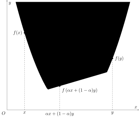
Convex Function on
A function is called a convex function if, for every and , it satisfies
We call a convex function, where the arithmetic rules for specify that multiplying by any positive real number, or adding any real number to it, gives itself, and that for every real , .
If the inequality is replaced by , the function is correspondingly called concave1. Since is concave, is convex, so this section considers only convex functions.
Only Proper Convex Functions Are Considered
To avoid discussing the value of and additional technical complications, whenever concepts related to convex functions are discussed, we assume that the function never takes the value and is not identically . Such a function is called a proper convex function. This is sufficient for understanding the algorithmic content of programming competitions.
In general, a function need not be defined for every real number. If the domain of is only a subset of , extend it to a function on as follows:
Then is called convex if and only if the corresponding satisfies the definition above. Thus, unless stated otherwise, the domain of every convex function mentioned in this article is the real line . Clearly, a convex function can take finite values only on an interval, that is, a convex subset of .
Simple Examples
Common examples of convex functions include:
- A constant function: , where ;
- A linear function: , where and ;
- The absolute-value function: , where ;
- The restriction of any convex function to an interval, such as (also called the indicator function of in the context of convex analysis).
More complicated convex functions can of course be built by combining the convexity-preserving transformations described below.
Convex Functions on Discrete Point Sets
In algorithm competitions, many functions are defined only at some integer points. In general, they are not convex functions in the sense defined above, because their domains are no longer convex sets. To handle this situation, convexity for functions on a discrete point set must be defined separately. In brief, first linearly interpolate the function, extending its domain to an interval, and then test its convexity.
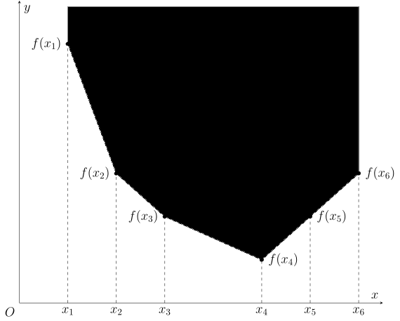
Convex Function on a Discrete Point Set
Let be a discrete point set, meaning that for every closed interval , is finite. For a function , define a function as follows:
-
When , set ;
-
when , let and , and set
-
when , set .
Then, if is convex on , is called convex on .
Because convex functions on are easier to work with, this article uses “convex function” to mean a function on unless stated otherwise. If a function in this article is given only at some integer points, its values at other real points are determined by the in the definition; equivalently, we are directly considering the corresponding piecewise-linear function .
Convex functions on the integers have a more intuitive equivalent definition:
Equivalent Definition of Convexity on
A function is convex if and only if
holds for every .
Proof
This proposition is a direct consequence of the slope characterization of convex functions.
If is convex on , then the slopes are nondecreasing, so
This is exactly the condition above.
Conversely, if the condition above holds, then for any ,
This is the arithmetic mean of all differences satisfying . Increasing by one inserts a larger difference, while increasing by one removes a smallest difference. Both operations increase the mean. This shows that the slope is nondecreasing, so is convex on .
In other words, any sequence whose slopes (differences) are nondecreasing can be regarded as a convex function on .
Two Characterizations of Convex Functions
The slope characterization of convex functions can in fact be generalized to the general case.
Slope Characterization of Convex Functions
Let be or a discrete subset of it. Then a function is convex if and only if its slope
For every with , this slope is a nondecreasing function of and .
Proof
For a function on , written , and for , let and . Then
is equivalent to
Both inequalities are equivalent to , which is precisely the convexity of .
For a function on restricted to a discrete subset , written , the necessity of nondecreasing slopes follows from the convexity of . To prove sufficiency, it is enough to show that is also nondecreasing. Let with strictly increasing in , and suppose and . Naturally, . Let . We can show that .
There are two cases. If , then , so the inequality is immediate. Otherwise,
Since the slopes on are increasing, increases with , and therefore .
Using this result, take and , let , and choose such that . Then
Substituting the expression for gives the convexity of .
Nondecreasing slopes can be viewed as an equivalent definition of convexity. Precisely because convex-function slopes are monotone, maintaining slopes commonly requires data structures such as a heap (priority queue) or a balanced tree.
Another equivalent characterization will also be useful. For , consider the region above the graph of the function in the plane:
This region is also called the epigraph of . Convexity of the function is equivalent to convexity of its epigraph:
Epigraph Characterization of Convex Functions
A function is convex if and only if is a convex set in .
Proof
If is convex, then for and any ,
Therefore, .
Conversely, if is convex, then for any and ,
This is equivalent to , which is the convexity of .
As we will see later, epigraphs connect the infimal convolution of convex functions with the Minkowski sum of convex sets.
Transformations of Convex Functions
We now introduce several convexity-preserving transformations that frequently occur in Slope Trick.
Nonnegative Linear Combinations
For convex functions and and nonnegative real numbers , the function is also convex. Moreover,
Thus, if the slopes of convex functions and are maintained, the slopes of their nonnegative linear combination can be obtained by computing each segment separately.
In slope-maintenance problems, one of the functions often has a simple form, in which case lazy tags can reduce the update complexity. In kink-maintenance problems, finding the slope kinks of only requires merging the slope kinks of and .
Infimal Convolution (Minkowski Sum)
Another common operation on convex functions is infimal convolution. For functions and , define
and call the infimal convolution2 of and . If and are both convex, their infimal convolution is also convex.
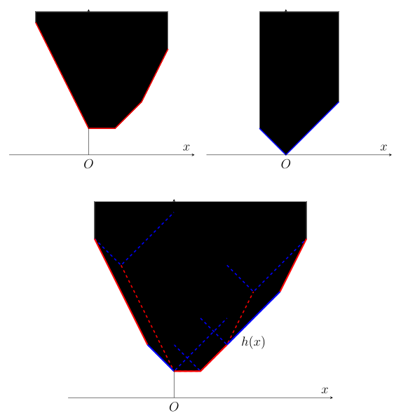
Interpreting the Illustration
To find the infimal convolution of and , namely , regard every point on the graph of (the red dashed curve in the third panel) as the origin and draw a graph of in the corresponding coordinate system (the blue dashed curve in the third panel). As the origin of the coordinate system moves along the graph of , the outline traced by the moving graph of (its epigraph), namely the lower convex hull, is the graph of . Thus, every slope segment of is either a slope segment of or one of ; the segments have simply been reordered by slope. The roles of and may be exchanged: moving the graph of along the graph of gives the same result.
Geometrically, is the Minkowski sum of and . If and are piecewise-linear functions, then is also piecewise linear, and its slope segments can be viewed as the result of merging and then sorting the slope segments of and .
Proof
Let be convex and let be their infimal convolution. Take and . By the definition of infimal convolution, for any , there exist such that and
Combining this with the convexity of and the definition of gives
Since is arbitrary,
This proves the convexity of .
For the geometric statement, strictly speaking, we can prove only
Here denotes closure.
For any , there are and with and
Hence , proving .
Conversely, for any , we have . By the definition of , for every there are such that
Let and , so . Thus, for every , a point lies on the line segment joining and . Letting yields .
Therefore, if and only if it is a closed convex set. One sufficient condition is that and are proper, convex, and lower semicontinuous. This is enough for algorithmic applications; piecewise-linear functions, for example, always satisfy these conditions.
In practice, if one of and has fewer slope segments, we can insert the shorter list directly into the longer one. Otherwise, small-to-large merging, a meldable heap, or another problem-specific technique may be needed to reduce the overall merge complexity, or an appropriate method may need to be found for the specific problem.
Minimum and Maximum Operations
The maximum of two convex functions is still convex, but the minimum of two convex functions need not be convex.
Many common minimum operations can be transformed into infimal convolution:
Examples
-
is still convex, because it can be written as the infimal convolution
-
is convex on if is convex on and the function defined on the finite set , , is convex on that discrete set. Indeed, after extension, can be viewed as the infimal convolution
Therefore, the function before extension is also convex.
However, not every minimum operation preserves convexity.
Counterexample
Let be convex. The function need not be convex.
In some special problems, although the DP transition can be written as the minimum of two convex functions and is difficult to transform into an infimal convolution, the value function nevertheless remains convex. In practice, it is usually necessary to combine tabulation with conjectures to find a suitable slope transition method for such problems.
After understanding convex functions and their common transformations, we can understand Slope Trick DP optimization through specific problems. The example problems in this article are roughly divided into two groups, maintaining kinks and maintaining slopes, to illustrate common operations and implementation details for these two methods. However, as emphasized above, the maintenance method is not the essence of Slope Trick; an appropriate way to maintain slope segments should be chosen according to the needs of the specific problem.
Maintaining Kinks
These problems usually arise when the goal is to minimize a sum of absolute values. Because the absolute value of the value function's slope is not large in such problems, it is more convenient to maintain the points where the slope changes.
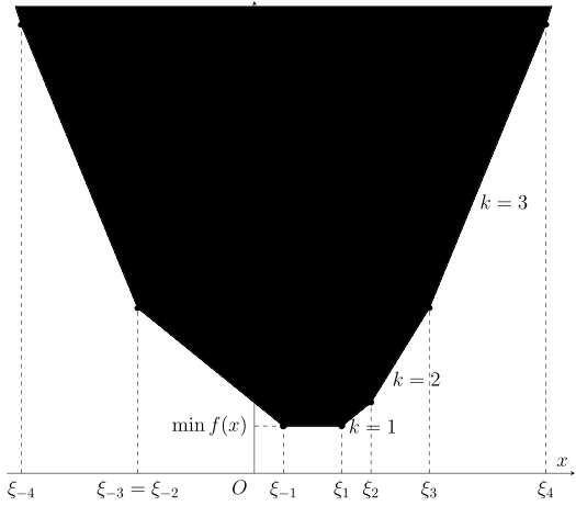
Maintaining kinks means maintaining the points at which the slope changes in a piecewise-linear function. Equivalently, for every slope on segment , maintain only its endpoints; the slope itself need not be stored separately. Therefore, whenever the slope changes in this type of problem, it should change only by a fixed amount. For example, if we maintain the kink set , this means that on , the slope is ; moving left across each kink decreases the slope by one, while moving right across each kink increases it by one. Thus, the slope on is , the slope on is , and so on. In formal notation, the function can be written using its slope kinks as
Its minimum is , and is attained at every point in .
Example: Minimum-Cost Increasing Sequence
[BalticOI 2004] Sequence
Given a sequence of length , , find a strictly increasing sequence minimizing , and output the minimum value and any optimal solution .
Solution
First, being strictly increasing is equivalent to being nondecreasing. Therefore, from we can find a nondecreasing sequence minimizing the difference, and then recover .
Consider the naive DP solution. Let be the minimum difference after selecting the first values of —there are of them—and requiring the -th value to be no greater than , compared with , taking its first values:
The state transition is readily obtained:
The initial state is , and the final answer is . Using the transformations of convex functions introduced above, transforming into requires two steps:
- First, add . This increases all slope segments in by and all slope segments in by .
- Take the minimum of the resulting function, changing into . From the analysis above, this is equivalent to taking the infimal convolution of and . The latter has only one slope segment, with slope extending infinitely to the right. Inserting it into the slope segments of is equivalent to deleting all positive-slope segments.
Once these operations are clear, all slope segments can be maintained directly with a balanced tree, but the code is complicated. Notice that the slope changes by at most each time in this problem, so the absolute value of every slope is at most . Instead of maintaining slope segments directly, it is more convenient to maintain the slope kinks.
Suppose the kink set of is . Then the two operations above correspond to:
- Add a kink at for a negative-slope segment and a kink at for a positive-slope segment.
- Pop the kinks of all positive-slope segments.
In the actual maintenance, after each operation there are no kinks of positive-slope segments, so the slope kinks have the form . Moreover, the operations always occur at the boundary between positive- and negative-slope segments, so it is enough to maintain a max-heap containing all kinks. The two operations correspond to:
- Insert twice.
- Pop the top of the heap.
Of course, the minimum value of the current function must also be maintained after each operation. Since there are no positive-slope kinks after an operation, the minimum is the value of the function at the top of the max-heap. Suppose the heap top before each operation is and the minimum is . Because the popped top is the smallest kink of the positive-slope segments, the minimum equals the function value at that point. Thus, we can directly compute the function value at the heap top before popping, namely
The equality of the first terms follows because has no positive-slope segments. Therefore, at each step we only need to repeatedly add to the minimum value.
This problem also asks us to output one optimal solution. At the end of the final operation, the optimal solution is the heap top, so the value of can be determined directly. If the -th optimal value is known and we need an optimal solution of satisfying , note that because is convex, the closer a point is to its global minimum point, the better the solution. Therefore, it is enough to record a global minimum point of and take its minimum with to obtain the optimal .
The time complexity is .
#include <iostream>
#include <queue>
#include <vector>

int main() {
  int n;
  std::cin >> n;
  std::vector<int> a(n), b(n);
  for (int& x : a) std::cin >> x;
  for (int i = 0; i < n; ++i) a[i] -= i;
  long long res = 0;
  std::priority_queue<int> max_heap;
  for (int i = 0; i < n; ++i) {
    max_heap.emplace(a[i]);
    max_heap.emplace(a[i]);
    res += max_heap.top() - a[i];
    max_heap.pop();
    b[i] = max_heap.top();
  }
  std::cout << res << '\n';
  for (int i = n - 2; i >= 0; --i) b[i] = std::min(b[i], b[i + 1]);
  for (int i = 0; i < n; ++i)
    std::cout << (b[i] + i) << (i == n - 1 ? '\n' : ' ');
  return 0;
}
Template problems:
- Codeforces 713 C. Sonya and Problem Without a Legend
- Luogu P2893 [USACO08FEB] Making the Grade G
- Luogu P4331 [BalticOI 2004] Sequence
- Luogu P4597 Sequence
- AtCoder 2nd Dwango Programming Contest Preliminary E - Fireworks
Example: The Case with a Bounded Transition
[NOISG 2018 Finals] Safety
Given a sequence of length , , find a sequence satisfying for all $1 [!note]- Solution
The content is broadly similar to the previous problem, except that the constraint on the sequence has changed. Likewise, let be the minimum difference when the -th value is , for the first values:
The state transition is
The initial condition is . The final answer is still .
Decompose the state transition into operations on convex functions. It has two steps:
- First take the minimum over , obtaining . This is the infimal convolution of and .
- Then add to the resulting function.
Again, because the slope changes by only one each time, we can consider maintaining kinks. The two operations can then be described as:
- Move all negative-slope segments units to the left, and all positive-slope segments units to the right.
- Insert twice.
For this problem, it is clearly convenient to maintain the positive- and negative-slope segments separately. Since the operations are concentrated mainly around the zero-slope segment, consider using a two-heaps structure, that is, a max-heap and a min-heap to maintain the kinks of the negative- and positive-slope segments. Apply the overall translation of the kinks in each heap with a lazy tag. The second operation needs to insert into each heap, and after the insertion the top of the max-heap may no longer be no greater than the top of the min-heap. In that case, swap the two heap tops until the ordering is restored.
Finally, consider how to update the minimum during the operations. The first translation operation does not change the minimum, so only the heap-top swaps need to be considered. Suppose . When the heap tops and are swapped, the function changes from
to
The function shape does not change during this process; it is only shifted downward by . Therefore, to keep the function unchanged before and after swapping the heap tops, it is enough to add to the minimum.
The algorithm still has time complexity , because after each element is added, the heap-top swap is performed at most once.
#include <iostream>
#include <queue>
#include <vector>

int main() {
  int n;
  long long h;
  std::cin >> n >> h;
  std::priority_queue<long long> max_heap;
  std::priority_queue<long long, std::vector<long long>, std::greater<>>
      min_heap;
  long long lt = 0, rt = 0;
  long long res = 0;
  for (; n; --n) {
    long long x;
    std::cin >> x;
    lt += h;
    rt += h;
    max_heap.emplace(x + lt);
    min_heap.emplace(x - rt);
    auto l = max_heap.top() - lt;
    auto r = min_heap.top() + rt;
    while (l > r) {
      max_heap.pop();
      min_heap.pop();
      res += l - r;
      max_heap.emplace(r + lt);
      min_heap.emplace(l - rt);
      l = max_heap.top() - lt;
      r = min_heap.top() + rt;
    }
  }
  std::cout << res << std::endl;
  return 0;
}
Template problems:
- Luogu P4272 [CTSC2009] Sequence Transformation
- Luogu P11598 [NOISG 2018 Finals] Safety
- AtCoder Beginner Contest 217 H - Snuketoon
- AtCoder Regular Contest 070 E - NarrowRectangles
- AtCoder Regular Contest 123 D - Inc, Dec - Decomposition
Maintaining Slopes
For some other problems, maintaining slopes is more convenient. Such problems can often also be solved using the idea of regretful greedy or simulated min-cost flow. In the min-cost flow model, the minimum cost is often a convex function of the flow, which provides the foundation for using Slope Trick.
Example: Stock Trading
Codeforces 865 D. Buy Low Sell High
Given days of stock prices , all positive, with an initial holding of . Each day, one share may be bought, one share may be sold, or no trade may be made. Find the maximum profit after days.
Solution
First consider the naive DP solution. Let be the maximum profit after day when holding shares:
The initial state is , and for every , . The answer is .
Transforming into requires two steps:
-
Take the supremal convolution of with the piecewise-linear function corresponding to
(which is clearly concave);
-
This gives the function finite values on , which conflicts with the requirement , so take only the part of the function on .
Translated into changes to slope segments, these are:
- Insert a slope segment of length and slope ;
- Delete, among the slope segments with finite slope, the segment with the largest slope and length .
Since the lengths of slope segments are always integers, we may maintain several slope segments of length one and record only the slope of each segment. Since we only need insertion and maximum queries, a max-heap is enough. The two operations are:
- Insert twice.
- Pop the heap top.
We also need to maintain the value of . The function obtained after the first operation has value at equal to , so its value at is that value plus the heap top that is about to be popped, which is the slope of the function on . Because truncation does not change the value at , this is .
Comparing this implementation with the code for Minimum-Cost Increasing Sequence above shows that this algorithm is equivalent to finding the minimum cost of changing the stock prices into a nonincreasing sequence.
The time complexity is .
#include <iostream>
#include <queue>
#include <vector>

int main() {
  int n;
  std::cin >> n;
  std::vector<int> a(n);
  for (int& x : a) std::cin >> x;
  long long res = 0;
  std::priority_queue<int> max_heap;
  for (int x : a) {
    max_heap.emplace(-x);
    max_heap.emplace(-x);
    res += x + max_heap.top();
    max_heap.pop();
  }
  std::cout << res << '\n';
  return 0;
}
Template problem:
Example: Moving Soil and Stones
[USACO16OPEN] Landscaping P
Given sequences of length , and , representing the amount of soil already in and the amount of soil required by garden , respectively (neither extra soil nor a shortage is allowed). Buying one unit of soil and putting it in any garden costs , removing one unit of soil from any garden costs , and transporting one unit of soil from garden to garden costs . Find the minimum cost of satisfying all garden demands. (.)
Solution
Consider the naive DP solution. Let be the minimum cost after satisfying the demands of the first gardens, when a net surplus of units of soil is transported to later gardens. If , this means that a net shortage of units must be transported from later gardens. Then the state transition can be written as
Here, denotes the cost when the net amount of soil purchased for the current garden is :
This is clearly convex. The meaning of the state transition is:
- When the net surplus of soil among the first gardens is , the minimum cost is .
- The cost of transporting the net surplus (or shortage) between gardens and is .
- By buying and selling, the amount of soil in garden is adjusted from to , and the net surplus is adjusted from to , at minimum cost .
The initial state is , and for every , . The answer is .
Transforming into can be divided into three steps:
- First, add , obtaining .
- Then take the infimal convolution with , obtaining .
- Finally, shift the function units to the left.
Converted into operations on slope segments, the three steps are:
- Add to all slope segments left of the origin, and add to all slope segments right of the origin.
- Replace every slope segment smaller than by , and every slope segment greater than by .
- Shift all slope segments units to the left.
In the original problem, and are small, so it is enough to maintain several slope segments of length . Although there are infinitely many slope segments, their upper and lower bounds are and , and there are only a few segments strictly between them. Since there are no insertion operations, two stacks can maintain the slope segments on the two sides of the origin, with interval additions and interval extrema handled by lazy tags. The three operations above correspond to:
- Apply lazy tags to the two stacks, adding on the left and on the right.
- Whenever an element is popped from a stack, take its maximum with and its minimum with . If the left stack is empty, pop ; if the right stack is empty, pop .
- Pop elements from the top of the left stack and insert them into the right stack; when , do the reverse.
When swapping stack tops, update the answer: moving left subtracts the current slope, while moving right adds the current slope.
The algorithm has complexity .
#include <iostream>
#include <stack>

int main() {
  int n;
  long long x, y, z;
  std::cin >> n >> x >> y >> z;
  std::stack<long long> neg, pos;
  long long lt = 0, rt = 0;
  long long res = 0;
  for (; n; --n) {
    int a, b;
    std::cin >> a >> b;
    lt -= z;
    rt += z;
    for (; b < a; ++b) {
      auto l = -y;
      if (!neg.empty()) {
        l = std::max(l, neg.top() + lt);
        neg.pop();
      }
      pos.emplace(l - rt);
      res -= l;
    }
    for (; b > a; --b) {
      auto r = x;
      if (!pos.empty()) {
        r = std::min(r, pos.top() + rt);
        pos.pop();
      }
      neg.emplace(r - lt);
      res += r;
    }
  }
  std::cout << res << std::endl;
  return 0;
}
Template problems:
- Luogu P2748 [USACO16OPEN] Landscaping P
- Kyoto University PC 2016 H - WAAAAAAAAAAAAALL
- JAG Practice Contest 2017 J - Farm Village
Problems for Practice
This article concludes with some problems from algorithm competitions that can be solved using Slope Trick, for practice.
- Luogu P3642 [APIO2016] Fireworks
- Luogu P9962 [THUPC 2024 Preliminary] A Tree
- Luogu P11317 [RMI 2021] Paths
- AtCoder Beginner Contest 383 G - Bar Cover
- Codeforces 280 D. k-Maximum Subsequence Sum
- Codeforces 280 E. Sequence Transformation
- Codeforces 802 O. April Fools' Problem (hard)
- Codeforces 1209 H. Moving Walkways
- Codeforces 1229 F. Mateusz and Escape Room
- Codeforces 1534 G. A New Beginning
- Codeforces 1787 H. Codeforces Scoreboard
- 2019 Summer Petrozavodsk Camp H. Honorable Mention
- 2018 ACM-ICPC World Finals C. Conquer The World
- 300iq Contest 3 F. Farm of Monsters
References and Notes
- [Tutorial] Slope Trick - zscoder
- Slope trick explained - Kuroni
- Slope Trick - USACO Guide
- [Tutorial] Intuition on Slope Trick - maomao90