AIOJ

在数理逻辑中，布尔代数（boolean algebra）是代数的一个分支．初等代数中变量的值是数字，其研究的主要运算符有加法、乘法、乘方以及这三种运算的逆运算．而布尔代数中变量的值仅为真和假两种（通常记作 $1$ 和 $0$ ），其研究的主要运算符有合取（与， $\land$ ）、析取（或， $\lor$ ）、否定（非， $\lnot$ ）．就像初等代数是描述数字运算的一种形式一样，布尔代数是描述逻辑运算的一种形式．

布尔函数

定义

布尔函数（boolean function）指的是形如 $f:\mathbf{B}^k\to \mathbf{B}$ 的函数，其中 $\mathbf{B}=\{0,1\}$ 为 布尔域（boolean domain），非负整数 $k$ 为该布尔函数的元数（arity）． $k=1$ 的布尔函数为一元函数，以此类推． $k=0$ 时，我们认为函数退化为 $\mathbf{B}$ 中的常量．

我们一般只研究一元和二元的布尔函数．如无特殊说明，下文的布尔函数仅限于一元和二元的情况．

除了函数的一般表达方式外，我们还可以用 真值表（truth table）、逻辑门（logic gate）、Venn 图来表示布尔函数．

真值表

对一个布尔函数，我们枚举其输入的所有情况，并将输入和对应的输出列成一张表，这个表就叫做真值表．

$n$ 元布尔函数也可以用含 $n$ 个变量的 命题公式（propositional formula）表示，命题公式 $p$ 与 $q$ 逻辑等价（logically equivalent）当且仅当其描述的是同一个布尔函数，记作 $p\iff q$ ．

以下是一些常见布尔函数，我们也会把这些布尔函数统称为 逻辑运算符（logical connective）或 逻辑算子（logical operator）：

名称（数理逻辑）	其他名称	记号
恒真（truth、tautology）		$\top$
恒假（falsity、contradiction）		$\bot$
命题	自身	$A$
否定（negation）	非（NOT）	$\lnot A$
合取（conjunction）	与（AND）	$A \land B$
析取（disjunction）	或（OR）	$A \lor B$
非合取（non-conjunction）	与非（NAND）、Sheffer 竖线	$A \bar{\land} B$ 、 $A\uparrow B$
非析取（non-disjunction）	或非（NOR）	$A \bar{\lor} B$ 、 $A\downarrow B$
	异或（Exclusive-OR，XOR）	$A \oplus B$
	同或（Exclusive-NOR）	$A \odot B$
实质蕴含（material implication）¹		$A \to B$
实质非蕴含（material nonimplication）¹		$A \nrightarrow B$
反蕴涵（converse implication）¹		$A \gets B$
非反蕴涵（converse nonimplication）¹		$A \nleftarrow B$
双条件（biconditional）、等价（equivalence）¹²		$A \leftrightarrow B$
非等价（non-equivalence）¹³		$A \nleftrightarrow B$

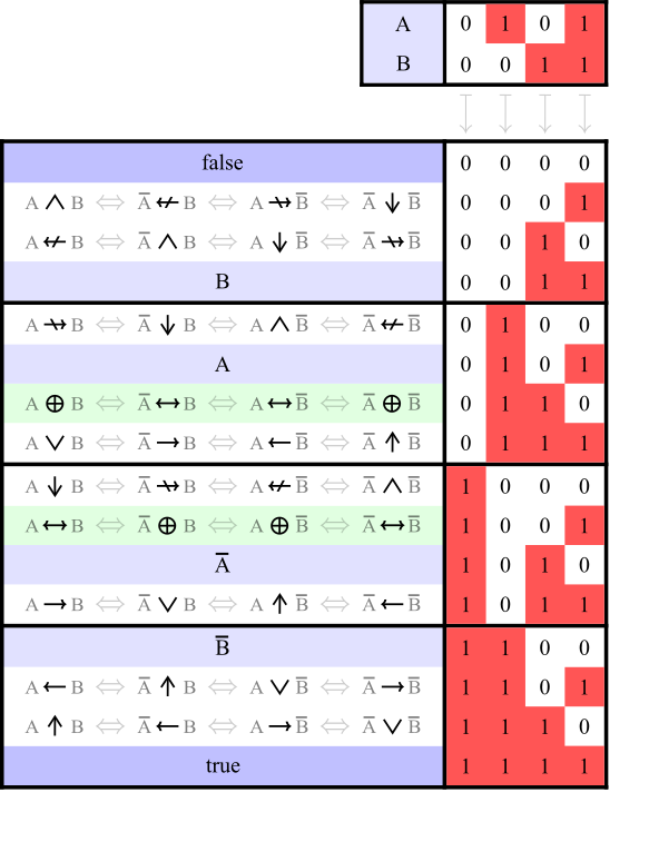
对应的真值表（From Wikipedia）：

$配图：logical connectives table$

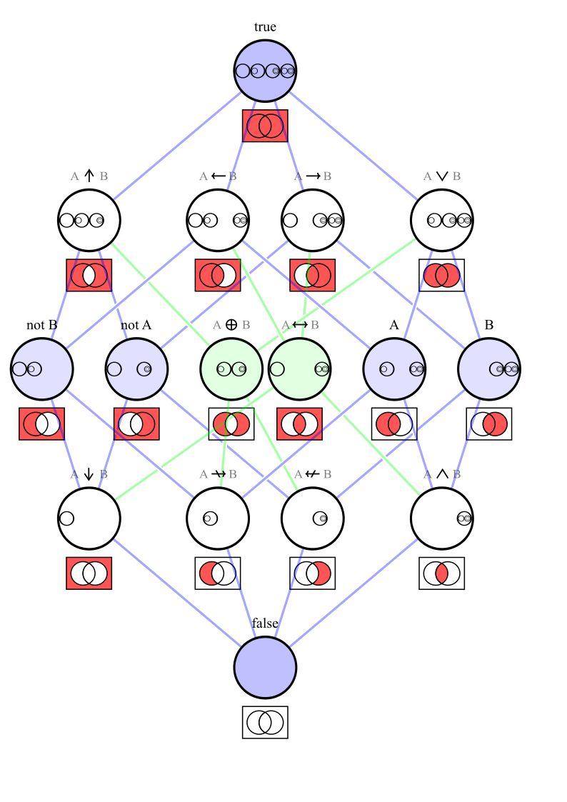
对应的 Venn 图和 Hasse 图（以集合的包含关系 $\subseteq$ 为偏序，From Wikipedia）：

$配图：logical connectives hasse diagram$

由于 $n$ 元布尔函数的输入有 $2^n$ 种，所以 $n$ 元布尔函数有 $2\uparrow (2\uparrow n)$ 种，其中 $\uparrow$ 为 Knuth 箭头．

我们把逻辑算子的组合称为 逻辑表达式（logical expression）．

如果我们把 $\mathbf{B}$ 视作模 $2$ 的一个剩余类，此时异或等价于模 $2$ 加法，与等价于模 $2$ 乘法，所以有时我们也用 $\mathbf{Z}_2$ 表示布尔域．

优先级

一元逻辑算子优先级高于二元逻辑算子，即 $\lnot$ 的优先级高于 $\land$ 、 $\lor$ 、 $\oplus$ 等的优先级．

二元逻辑算子之间的优先级有多种规定，有的资料认为 $\land$ 、 $\lor$ 、 $\oplus$ 的优先级比 $\to$ 、 $\gets$ 、 $\leftrightarrow$ 更高，而有的资料持相反观点．所以在使用时推荐多加括号来明确顺序．

C++ 中的规定参见 C++ 运算符优先级总表．

自足算子与完备算子集

实际上，我们只用与非或者或非即可表达其余的逻辑算子，CPU 也是基于这一点构建的．但是，由于 与、或、非、异或 这四种逻辑算子的性质更好，所以我们在研究布尔代数时一般只使用这四种函数．

如何分别用与非、或非表示其余的逻辑算子

我们有

$\lnot p=p\bar{\land} p=p\bar{\lor} p$ ，
$p\land q=(p\bar{\land}q)\bar{\land}(p\bar{\land}q)=(p\bar{\lor}p)\bar{\lor}(q\bar{\lor}q)$ ，
$p\lor q=(p\bar{\land}p)\bar{\land}(q\bar{\land}q)=(p\bar{\lor}q)\bar{\lor}(p\bar{\lor}q)$ ，
$p\to q=p\bar{\land} (q\bar{\land} q)=((p\bar{\lor}p)\bar{\lor}q)\bar{\lor}((p\bar{\lor}p)\bar{\lor}q)$ ．

另外

$p=\lnot\lnot p$ ，
$p\nleftrightarrow q=p\oplus q=(p\lor q)\land\lnot (p\land q)$ ，
$p\leftrightarrow q=p\odot q=\lnot(p\oplus q)$ ，
$p\nrightarrow q=\lnot(p\to q)$ ，
$p\gets q=q\to p$ ，
$p\nleftarrow q=\lnot(p\gets q)$ ．

我们能不能用指定的若干逻辑算子描述所有的逻辑算子？这便引出了完备算子集的定义．

定义

对一个给定的逻辑算子集，如果能只用这个集合里的函数描述所有的逻辑算子，则称该集合为 完备算子集（functionally complete operator set）．特别地，如果只用一个逻辑算子即可描述所有的逻辑算子，则称该算子为 自足算子（sole sufficient operator）或 Sheffer 函数（Sheffer function）．

如果在一个完备算子集中删去任意一个元素，其都不能描述所有的逻辑算子，则称该集合为 极小完备算子集（minimal functionally complete operator set）．

可以证明逻辑算子中只有 $\bar{\land}$ 、 $\bar{\lor}$ 是自足算子．

以下为常见的极小完备算子集⁴：

$\{\bar{\land}\}$ ， $\{\bar{\lor}\}$ ，
$\{\land,\lnot\}$ ， $\{\lor,\lnot\}$ ， $\{\gets,\lnot\}$ ， $\{\to,\lnot\}$ ， $\{\nleftarrow,\lnot\}$ ， $\{\nrightarrow,\lnot\}$ ，
$\{\gets,\bot\}$ ， $\{\to,\bot\}$ ， $\{\nleftarrow,\top\}$ ， $\{\nrightarrow,\top\}$ ，
$\{\gets,\nleftarrow\}$ ， $\{\to,\nleftarrow\}$ ， $\{\gets,\nrightarrow\}$ ， $\{\to,\nrightarrow\}$ ，
$\{\gets,\nleftrightarrow\}$ ， $\{\to,\nleftrightarrow\}$ ， $\{\nleftarrow,\leftrightarrow\}$ ， $\{\nrightarrow,\leftrightarrow\}$ ，
$\{\lor,\leftrightarrow,\bot\}$ ， $\{\lor,\leftrightarrow,\nleftrightarrow\}$ ， $\{\lor,\nleftrightarrow,\top\}$ ，
$\{\land,\leftrightarrow,\bot\}$ ， $\{\land,\leftrightarrow,\nleftrightarrow\}$ ， $\{\land,\nleftrightarrow,\top\}$ ．

性质

首先是代数结构的相关性质：

与、或均关于 $\mathbf{B}$ 构成交换幺半群．即与运算和或运算均具有交换律、结合律和幺元（ $x\land 1=x\lor 0=x$ ）．
异或、同或均关于 $\mathbf{B}$ 构成群．即异或运算和同或运算均具有交换律、结合律、幺元（ $x\oplus 0=x\odot 1=x$ ）和逆元（ $x\oplus x=0$ ， $x\odot x=1$ ）．
与非、或非均不具有结合律，所以不构成半群．

对于 $\land$ 、 $\lor$ ，我们有

分配律：
- $a\land(b\diamond c)=(a\land b)\diamond (a\land c)$ ，其中 $\diamond$ 可以为 $\land$ 、 $\lor$ 、 $\oplus$ ，
- $a\lor(b\diamond c)=(a\lor b)\diamond (a\lor c)$ ，其中 $\diamond$ 可以为 $\land$ 、 $\lor$ 、 $\odot$ ．
幂等（idempotence）律： $x\land x=x$ 、 $x\lor x=x$ ．
单调性： $a\to b\iff(a\land c)\to(b\land c)$ 、 $a\to b\iff(a\lor c)\to(b\lor c)$ ．
吸收（absorption）律： $x\land(x\lor y)=x\lor(x\land y)=x$ ．
与「 $\to$ $\to$ 」的关系：
- $a \lor b \iff (\lnot a \to b) \land (\lnot b \to a)$ ，
- $a \land b \iff \lnot((a \to \lnot b) \lor (b \to \lnot a))$ ．

布尔函数的单调性

对一个布尔函数 $f(x_1,\dots,x_n)$ 和 $\mathbf{B}^n$ 中的两个元素 $(a_1,\dots,a_n),(b_1,\dots,b_n)$ ，若当 $a_i\leq b_i,~~\forall i=1,\dots,n$ 时恒有 $f(a_1,\dots,a_n)\leq f(b_1,\dots,b_n)$ ，则称该布尔函数是单调的．

我们还有如下性质：

排中律（law of excluded middle）： $p\lor\lnot p$ 恒真．
$\lnot p\iff p\to\bot$ ．
双重否定/ $\lnot$ 的对合（involution）律： $\lnot\lnot x=x$ ．
$\oplus$ 、 $\odot$ 的对合律： $x\oplus y\oplus y=x$ 、 $x\odot y\odot y=x$ ．
De Morgan 律： $\lnot(p\land q)=\lnot p\lor \lnot q$ 、 $\lnot(p\lor q)=\lnot p\land \lnot q$ ．

逻辑表达式的标准化

根据上述性质，我们可以对逻辑表达式进行一定的等价变换，使其符合特定的范式，这一点可用于自动定理证明中．常见的标准化范式有 合取范式（conjunctive normal form，CNF）、析取范式（disjunctive normal form，DNF）和 代数范式（algebraic normal form，ANF）．

合取范式与析取范式

我们做如下递归式的定义：

文字（literal）：对变量 $x$ ， $x$ 和 $\lnot x$ 是文字．
子式：
- 文字是子式，
- 若 $A$ 是文字、 $B$ 是子式，则 $A\lor B$ 是子式．
合取范式：
- 若 $A$ 是子式，则 $(A)$ 是合取范式，
- 若 $A$ 是子式、 $B$ 是合取范式，则 $(A)\land B$ 是合取范式．

类似地，交换上面定义中的 $\land$ 与 $\lor$ 即可得到析取范式的定义．

例如以下逻辑表达式均为析取范式：

$(A\land\lnot B)\lor(C\land D\land\lnot E)$ ，
$(A\land B)\lor (C)$ ，
$(A\land B)$ ，
$(A)$ ．

以下逻辑表达式均为合取范式：

$(\lnot A\lor\lnot B\lor C)\land(\lor D\lor\lnot E)$ ，
$(A\lor B)\land (C)$ ，
$(A\lor B)$ ，
$(A)$ ．

以下逻辑表达式既不为合取范式也不为析取范式：

$\lnot(A\land B)$ ，
$A\land (B\lor (C\land D))$ ．

我们可以通过如下的步骤将任意一个只含有 $\lnot$ 、 $\land$ 、 $\lor$ 运算的逻辑表达式变形为 DNF：

\begin{array}{rcccl} \lnot\lnot x &&\mapsto&& x,\\ \lnot(x\lor y) &&\mapsto&& \lnot x\land \lnot y,\\ \lnot(x\land y) &&\mapsto&& \lnot x\lor \lnot y,\\ x\land(y\lor z) &&\mapsto&& (x\land y)\lor (x\land z),\\ (x\lor y)\land z &&\mapsto&& (x\land z)\lor (y\land z). \end{array}

要得到表达式 $X$ 的 CNF，只需得到 $\lnot X$ 的 DNF 后取反并应用 De Morgan 律即可．

代数范式

首先，我们用如下递归式的定义来定义子式：

变量 $x$ 是子式，
若 $A$ 是子式， $x$ 是变量，则 $x\land A$ 是子式．

则满足如下三种形式之一的逻辑表达式为代数范式：

$1$ 、 $0$ ，
若干不等价子式的异或，如 $a\oplus b\oplus(a\land b)\oplus(a\land b\land c)$ ，
若干不等价子式与唯一的 $1$ 的异或，如 $1\oplus a\oplus b\oplus(a\land b)\oplus(a\land b\land c)$ ．

注意到代数范式和 $\mathbf{Z}_2$ 上的多项式一一对应，所以代数范式也被称为 Zhegalkin 多项式（Zhegalkin polynomial）．

我们可以通过如下的步骤将任意一个只含有 $\lnot$ 、 $\land$ 、 $\lor$ 、 $\oplus$ 运算的逻辑表达式变形为 ANF：

$\oplus$ ：直接展开，如 $(1\oplus x)\oplus(1\oplus x\oplus y)=1\oplus x\oplus 1\oplus x\oplus y=y$ ，
$\land$ ：用分配律展开，如 $x\land(1\oplus x\oplus y)=(x\land 1)\oplus (x\land x)\oplus (x\land y)=x\oplus (x\land y)$ ，
$\lnot$ ：将 $\lnot x$ 用 $1\oplus x$ 代替，如 $\lnot(1\oplus x\oplus y)=1\oplus 1\oplus x\oplus y=x\oplus y$ ，
$\lor$ ：将 $x\lor y$ 用 $1\oplus((1\oplus x)\land(1\oplus y))$ 或 $x\oplus y\oplus (x\land y)$ 代替，如 $(1\oplus x)\lor(1\oplus x\oplus y)=1\oplus((1\oplus 1\oplus x)\land(1\oplus 1\oplus x\oplus y))=1\oplus x\oplus(x\land y)$ ．

参考资料与注释

Footnotes

用于命题推导时应使用双横长箭头，如 $A\implies B$ 、 $A\impliedby B$ 、 $A\iff B$ 等． ↩ ↩² ↩³ ↩⁴ ↩⁵ ↩⁶
等价于同或． ↩
等价于异或． ↩
Vaughan, H. E. (1942). Complete sets of logical functions.Transactions of the American Mathematical Society 51: 117–32. ↩